19. Implementing PSO
The purpose of this topic is to see an implementation of particle swarm optimization (PSO)
It is a simple implementation that incorporates no enhancements
The problem PSO is being applied to in this example is some arbitrary benchmark real number optimization problem
Despite how simple the implementation is, it will still perform well
19.1. Problem
PSO is often used for real/floating point number optimization
Any real number optimization problem would work, but there there exist several benchmark test functions
The goal is
Given some \(n\) dimensional real/floating point number function
The function takes \(n\) real/floating point numbers as arguments
The function returns a single real/floating point number
Find the arguments for the function that produces the smallest/largest output
Depending on if it is a minimization or maximization problem
19.1.1. Matyas Function
Here, the Matyas function is used
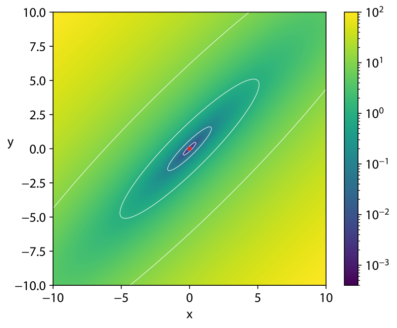
\(f(x, y) = 0.26(x^{2} + y^{2}) - 0.48xy\)
The optimal values for the function’s arguments are \((0, 0)\)
This function was arbitrary selected

Three-dimensional representation of the Matyas function. The function’s arguments (\(x, y\)) are represented in a two-dimensional Cartesian space and the function’s output, the third dimension, is represented by colour.
The Matyas function is used as a minimization problem that takes two arguments
Thus, the goal is to find the values of those arguments that result in the smallest value
Although it is known pre hoc that the optimal solution is \((0, 0)\)
The point is to see if PSO can find this solution
25def matyas_function(x, y):
26    """
27    Optimization function being searched through for the minimum value. This function's minimum value is at f(0,0) = 0
28    and has a search domain of -10 <= x,y <= 10. This function was taken from the wikipedia article on "Test functions
29    for optimization": https://en.wikipedia.org/wiki/Test_functions_for_optimization
30
31    :param x: X value
32    :param y: Y value
33    :return: Result of the matyas function
34    """
35    return 0.26 * (x**2 + y**2) - 0.48 * x * y
19.2. Initialization
Here, all particle positions and velocities are assigned random values to start
However, any form of initialization may be used
For example, seeding the particle positions with already known good points in space
40    particles = []
41    for _ in range(NUMBER_OF_PARTICLES):
42        particle = {
43            "position": np.random.uniform(START_POSITION_LOW_BOUND, START_POSITION_HIGH_BOUND, FUNCTION_DIMENSIONS),
44            "velocity": np.random.uniform(START_VELOCITY_LOW_BOUND, START_VELOCITY_HIGH_BOUND, FUNCTION_DIMENSIONS),
45        }
46        particle["best_known_position"] = particle["position"]
47        particles.append(particle)
48    global_best = particles[0]["position"]
Notice in the above code that the particles’ starting positions, although randomly selected, are bounded
Also notice that the particles’ best and global best positions are initialized
For reference, below are the hyperparameters selected
12FUNCTION_DIMENSIONS = 2
13START_POSITION_LOW_BOUND = -10
14START_POSITION_HIGH_BOUND = 10
15START_VELOCITY_LOW_BOUND = -0.1
16START_VELOCITY_HIGH_BOUND = 0.1
17NUMBER_OF_PARTICLES = 10
18ITERATIONS = 100
19INERTIA = 0.729844
20COGNITIVE = 1.496180
21SOCIAL = 1.496180
The inertia, social, and cognitive terms are set to the values suggested bu van den Bergh
The number of dimensions is dictated by the Matyas function
The other values are arbitrary selected
19.3. Evaluation
A particle’s position corresponds to the arguments that are to be provided to the function
Therefore, provide the particle’s coordinates to the function to evaluate
Once the function’s value is returned, update the particle’s best known position and global best position if necessary
Notice that each particle does not need to know what it’s fitness value is
The algorithm only cares about
Each particle’s best known position
The global best position
54        for particle in particles:
55            particle_value = matyas_function(*particle["position"])
56            if particle_value < matyas_function(*particle["best_known_position"]):
57                particle["best_known_position"] = particle["position"]
58            if particle_value < matyas_function(*global_best):
59                global_best = particle["position"]
19.4. Update Velocity & Speed
Once the random vectors for the cognitive and social terms are determined
63        for particle in particles:
64            r1 = np.random.rand(FUNCTION_DIMENSIONS)
65            r2 = np.random.rand(FUNCTION_DIMENSIONS)
66            particle["velocity"] = (
67                INERTIA * particle["velocity"]
68                + COGNITIVE * r1 * (particle["best_known_position"] - particle["position"])
69                + SOCIAL * r2 * (global_best - particle["position"])
70            )
71            particle["position"] = particle["position"] + particle["velocity"]
19.5. Termination Requirement
Any stopping criteria could be used
Here, a predetermined set of iterations was specified
In other words, the fitness and position update processes are repeated within a loop until all iterations complete
52    for _ in range(ITERATIONS):
53        # [begin-evaluation]
54        for particle in particles:
55            particle_value = matyas_function(*particle["position"])
56            if particle_value < matyas_function(*particle["best_known_position"]):
57                particle["best_known_position"] = particle["position"]
58            if particle_value < matyas_function(*global_best):
59                global_best = particle["position"]
60        # [end-evaluation]
61
62        # [begin-position-update]
63        for particle in particles:
64            r1 = np.random.rand(FUNCTION_DIMENSIONS)
65            r2 = np.random.rand(FUNCTION_DIMENSIONS)
66            particle["velocity"] = (
67                INERTIA * particle["velocity"]
68                + COGNITIVE * r1 * (particle["best_known_position"] - particle["position"])
69                + SOCIAL * r2 * (global_best - particle["position"])
70            )
71            particle["position"] = particle["position"] + particle["velocity"]
72        # [end-position-update]
Finally, once complete, the global best position will be the best position found by the PSO algorithm
76 print(global_best, matyas_function(*global_best))
19.6. For Next Class
TBD