17. Multi-Objective Problems
For the most part, all problems looked at have been single objective problems
However, it is not uncommon to have multiple objectives to optimize
Sometimes these objectives compliment each other, and sometimes they are in conflict with one another
Consider buying a house
Low price
Want at least 4 bedrooms
Want to have a small commute distance
Proximity to amenities
Style
Some of these features are subjective
Style
The amenities one cares about
Some complement one another
Small commute and amenities are probably related
Some are in conflict
At least 4 bedrooms and close to amenities
Low price
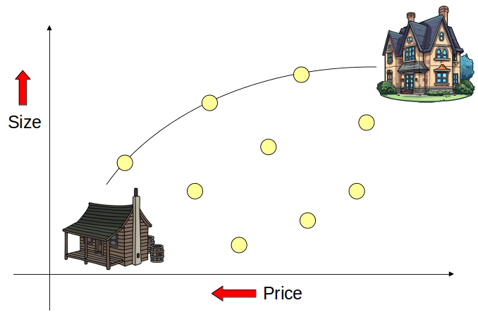
One may want a large house but to pay as little as possible. These objectives are in conflict with one another. Each point represents a potential house.
17.1. Scalarization
Scalarization is the process of scaling the various features to be optimized and combining them into a single value
It is a way to turn multi-objective problems into a single objective problem
It is an a priori process, meaning the decisions about the scaling must be done before the search starts
17.1.1. Weighted Sum
The simplest strategy is a weighted sum
Scale each individual objective being optimized and add them together to make a single value
\(w_{1}f_{1}(x) + w_{2}f_{2}(x) + w_{3}f_{3}(x) + ... + w_{m}f_{m}(x)\)
Or
\(\sum_{i}^{m}w_{i}f_{i}(x)\)
Where
\(x\) is some chromosome
\(m\) is the number of objectives being optimized
\(f_{i}(x)\) is a function returning the \(i^{th}\) objective’s fitness on chromosome \(x\)
\(w_i\) is the weight/scale of objective \(i\)
If one objective is more important than another, assign it a stronger weight
Use negative weights to account for objectives that are to be minimized/maximized
Unfortunately, however, weighted sums do not work too well beyond two or three objectives
Further, it’s not always easy to assign the weights
17.2. Dominance
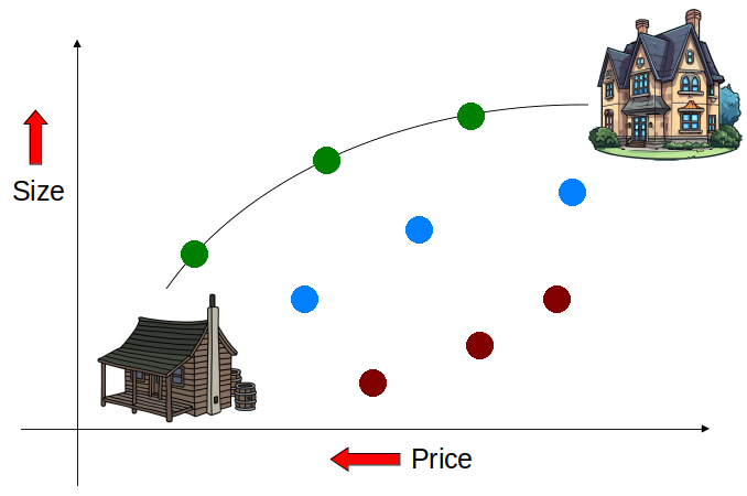
Given the goal of buying the largest house for as little as possible, it is difficult to pick a data point on the plot that is the “best” option. This is because it may be difficult to compare data points across dimensions (price vs. size). However, although it is difficult to select the “best” option, it may be simple to identify options that are better than others.
Sometimes it is not possible to truly select the best option
If one house has a lower price than another, then that’s good
And if one house is bigger than another, then that’s good
But, how does one compare price to size?
However, it may be clear that some options are better/worse than others
If a house is bigger and cheaper than another, then that’s good
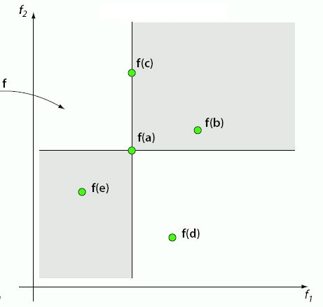
Five data points (a, b, c, d, e) for some two-dimensional minimization problem. Each dimension represents some objective to be minimized. Some data points are difficult to compare, but data points are “dominated” by other points.
In the above example,
Point a is better than b in both dimensions
Point a is better than c in one dimension, but equal in another
Point a is worse than e in both dimensions
It is difficult to compare points a and d since one is better in one dimension but worse in the other
Here, one would say point a dominates points b and c
Although a and c are equal along the x-axis, a is still better in the y-axis
Thus, one would still choose a as the better data point
Further, point a is dominated by point e
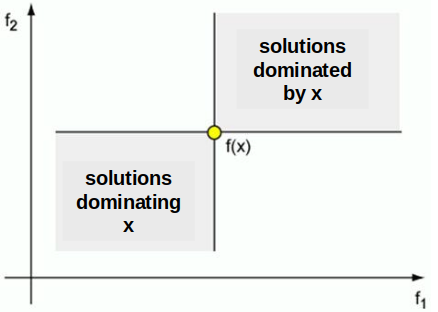
Portions of a two-dimensional space dominated by some data point x (top right — worse than x in both dimensions) and dominating data point x (bottom left — points that are better than x in both dimensions). The other portions of the space (top left/bottom right) are difficult to compare to x as they are better than x in one dimension but not the other.
17.2.1. Pareto Sets
Given the set of solutions \(S\) and some subset of solutions \(Q \subset S\)
A data point \(x \in S\) is non-dominated by the set \(D\) if no solution \(y \in D\) dominates \(x\)
A set of non-dominated solutions \(N \subset S\) defines the Pareto-Optimal Set
It is possible to create multiple Pareto Sets by repeatedly applying this process on the set difference \(S - N\)
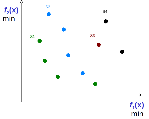
Data points in some two-dimensional minimization problem. Four Pareto Sets exist — S1, S2, S3, and S4. All solutions in S1 are non-dominated by any other solutions. All solutions in S2 are non-dominated by solution other than those in S1. Similarly for S3 and S4.
17.2.2. Evolutionary Algorithms and Pareto Style Multi-Objective Optimization
Since EC algorithms are typically population based, they work well with Pareto style multi-objective optimization
The population can be ranked into Pareto Sets
The Pareto-Optimal set will contain all good solutions
Consider the issue with weighted sum and selecting weights for difficult to quantify and compare feature
With a Pareto-Optimal Set, there is no need to decide on the weights
A set of solutions is presented in the end which can then be selected from
It may still be difficult to select a single solution from this Pareto-Optimal set
But at least that’s not something the algorithm is trying to figure out for the user
17.3. For Next Class
TBD