18. Particle Swarm Optimization

Particle Swarm Optimization (PSO) is a stochastic population based optimization technique
- Like many forms of evolutionary computation
It consists of particles that all act independently, but are influenced by the population

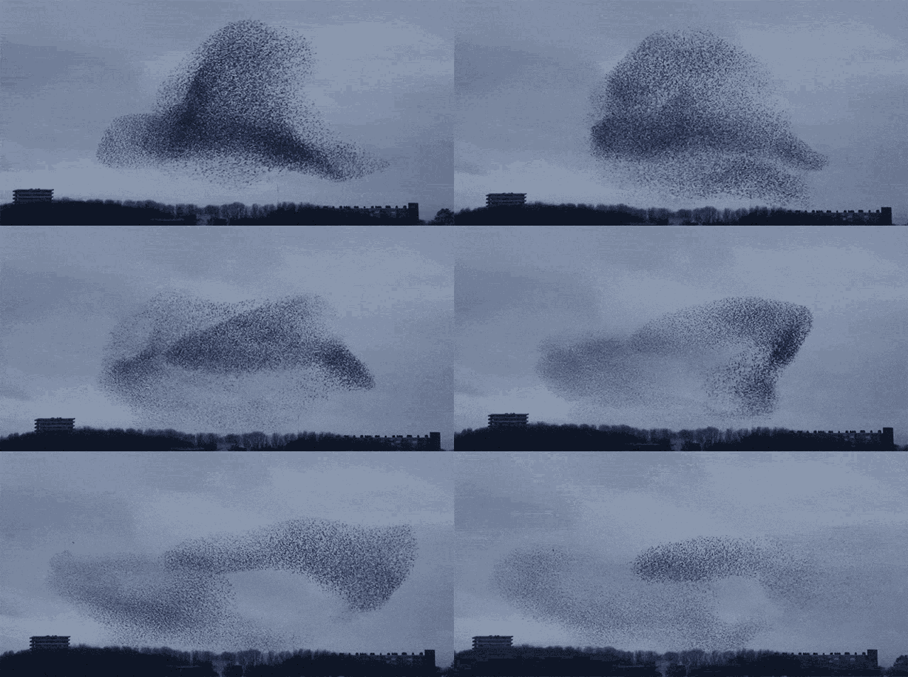
../../_images/birds_flying.gif — A flock of birds. Each bird is making decisions independently that are informed by other birds around them. As a result, it appears as if the flock is moving in some well coordinated way.

PSO is particularly well designed for real/floating point number optimization
It is relatively simple to implement compared to other forms of evolutionary computation
- It has relatively few hyperparameters to tune too
Further, it is simple to extend and enhance

18.1. Particles

PSO consists of a population of particles that represent points in some search space
- Like candidate solutions from a genetic algorithm
Unlike chromosomes, these particles do not have the traditional variation operators of mutation and crossover
Instead, the particles have a propensity to more towards areas that the particles likes
However, these particles are also influenced by the population of particles
- They also have a propensity to move towards areas that the population likes
In terms of an optimization problem
- Each particle has a propensity to move towards the best area of the search space it has encountered
- While also having a propensity to move to the best part of the search space the population has encountered
Each particle also has velocity and inertia

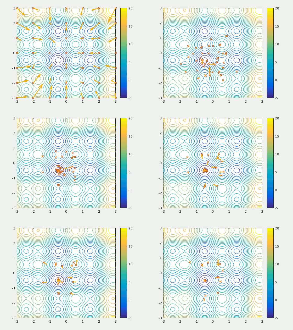
../../_images/particles_moving.gif — Particles moving through a two-dimensional space moving towards, in this example, points that minimize some function \(f(x, y)\). Arrows associated with each particle represents its velocity.

18.1.1. Representation

POS is often used for real/floating point number optimization
Thus, each particle is typically represented as an \(n\) dimensional vector encoding its position in space
- Where \(n\) is the dimensionality of the problem
- For example, in the above figure, each particle would be represented as a two-dimensional vector
- <1.42345478, -2.31345786555567>
Each particle has a
- Position in space, represented as an \(n\) dimensional vector containing a position in space
  \(\vec{x}(t)\) — Position at time \(t\)
- Velocity, which is also represented as an \(n\) dimensional vector containing deltas
  \(\vec{v}(t)\) — Velocity at time \(t\)
- Best visited position (\(n\) dimensional vector)
  \(\vec{p}_{best}\) — Particle’s best known position
- Access to the swarm’s best known position in space (\(n\) dimensional vector)
  \(\vec{g}_{best}\) — Global best known position

18.2. Velocity

The velocity determines where the particle will be for the next iteration of the algorithm
In other words, the velocity \(\vec{v}(t)\) is used to determine the position of particle \(\vec{x}(t+1)\)

18.2.1. Velocity Calculation

Velocities are typically initialized with some random values within some range
But as the algorithm executes, the velocity of the particles change as they become influenced by
- The particles’ best known position in space
- The population’s best known position in space

18.2.1.1. Inertia Term: \(\omega\vec{v_{i}}(t)\)

Each particle has some velocity
When particles’ velocities are being updated, the changes are applied to an already moving particle
These particles want to continue moving the way they are
- They resist change
Thus, the first part of a velocity update takes into consideration the current velocity of the particle
- \(\omega\vec{v_{i}}(t)\)
Where
- \(i\) is some particle
- \(\vec{v_{i}}(t)\) is the particle’s velocity at time \(t\)
- \(\omega\) is some coefficient use to control how much the particles want to resist change
  \(\omega \in [0, 1]\)

18.2.1.2. Cognitive Term: \(c_{1}\vec{r_{1}}(\vec{p_{i}}_{best} - \vec{x_{i}}(t))\)

Each particle wants to move towards the area of the search space it prefers
- The best known location for that particle
Thus, part of the velocity update alters the velocity such that it will move the towards this part of the space
- \(c_{1}\vec{r_{1}}(\vec{p_{i}}_{best} - \vec{x_{i}}(t))\)
Where
- \(i\) is some particle
- \(c_{1}\) is some coefficient used to control how much the particle is influenced by its best known position
  \(c_{1} \in [0, 2]\)
  
  The higher the \(c_{1}\), the more the particle is influenced by its best known position
- \(r_{1}\) is some stochastic vector discussed below
- \(\vec{p_{i}}_{best}\) is the particle’s best known position within the search space
- \(\vec{x_{i}}(t)\) is the particle’s position at time \(t\)
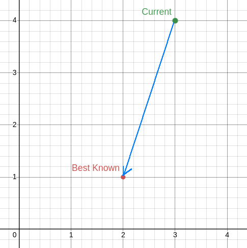
The difference between the particle’s best known position and current position dictates where the particle needs to go
- \(\vec{p_{i}}_{best} - \vec{x_{i}}(t)\)
\(c_{1}\) and \(r_{1}\) scale the vector

../../_images/plot_best_vs_current_position.png — Vector (blue) showing the difference between the particle’s best known position (red) and its current position (green). The vector \((-1, -3)\) is shown starting at the current position \((3, 4)\). If the particle were to have exactly this velocity for one time step, it would return to the best known position.

18.2.1.4. Random/Stochastic Components: \(\vec{r_{1}}\) and \(\vec{r_{2}}\)

The cognitive and social portions of the velocity update included the vectors \(\vec{r_{1}}\) and \(\vec{r_{2}}\) respectively
These vectors have values between \([0, 1]\) that are stochastically determined
- Randomly determined for each velocity update calculation for each particle
These random/stochastic vectors are important as they add a chance for novelty
Further, they have been empirically shown to improve the search and prevent premature convergence

18.2.1.5. Putting the Velocity Update Together

The velocity update is the sum of the parts of the update
- Inertia term + cognitive term + social term
Velocity update for some particle \(i\)

\[\vec{v_{i}}(t+1) = \omega\vec{v_{i}}(t) + c_{1}\vec{r_{1}}(\vec{p_{i}}_{best} - \vec{x_{i}}(t)) + c_{2}\vec{r_{2}}(\vec{g}_{best} - \vec{x_{i}}(t))\]

As discussed, there are three coefficients that need to be tuned for the algorithm
As a starting place, van den Bergh suggests
- \(\omega = 0.729844\)
- \(c_{1} = c_{2} = 1.496180\)
However, one should always aim to tune these values for their needs

18.3. Position Update

After the particle’s velocity is calculated, the particle’s new position can be determined
The new position is the sum of its current position and its current velocity

\[\vec{x_{i}}(t+1) = \vec{x_{i}}(t) + \vec{v_{i}}(t+1)\]

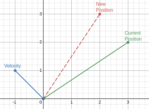
Consider the below figure
- The particle’s current position \(\vec{x_{i}}(t)\) is represented as the green vector
- The particle’s velocity \(\vec{v_{i}}(t+1)\) is represented as the blue vector
- The particle’s new position is represented as the red dashed vector
  The sum of the particle’s current position and velocity
  
  \((3, 2) + (-1, 1) = (2, 3)\)

../../_images/plot_position_update.png — The summation of the particle’s current position (green) and its velocity (blue) results in the particle’s new position within the search space (red). One could also visualize this by having the velocity vector start at the end of the current position vector (instead of the origin, as it is currently shown).

18.4. Algorithm

The high-level idea of the algorithm is presented below

Initialize the particles' positions randomly
Initialize the velocities randomly
While stopping criteria is not met
    For all particles
        Evaluate the particle's fitness
        Update particle's and global bests if necessary

    For all particles
        Calculate the particle's new velocity
        Update the particle's position

It may not be immediately obvious, but look for the similarities between this algorithm and a genetic algorithm
- Initialization
- Generational loop
- Fitness evaluation
- Variation operations
The major differences are that
- There is no real selection as all particles survive
  Although, this is a selection strategy
- The velocity and position updates are not mutation and crossover
  However, consider the cognitive and social aspects of the velocity update
  
  This is a mechanism for exploration and exploitation
  
  In other words, they are in fact variation operators

18.5. Simple Enhancements

PSO’s ability to be modified is one of the reasons it’s popular
- Like with most forms evolutionary computation, anything could be done
Some quick examples of some modifications are
- Neighbourhoods
  Each particle is part of some neighbourhood
  
  The neighbourhood’s best is also recorded and impacts the velocity updates
  
  \(c_{3}\vec{r_{3}}(\vec{n_j}_{best} - \vec{x_{i}}(t))\) is added to the velocity update calculation
  
  Where \(\vec{n_j}_{best}\) is the \(j^{th}\) neighbourhood’s best known location
  
  And \(c_{3}\) is some tunable constant and \(\vec{r_{3}}\) is another randomly determined vector
- Velocity clamping
  Disallow particles from having velocities over a certain value
  
  This could be done by setting a ceiling, or an exponentially decaying velocity
- Boundary/Position clamping
  Dissalow particles from going beyond some boundaries
  
  One could just set a limit and not allow particles beyond it
  
  More creative strategies include having particles jump to the other side of the space
  
  Or have the particles bounce off the boundary back in the other direction
- Charged PSO
  Particles repel one another
  
  The velocity update includes a term for the particles’ propensity to move away from one another

18.6. For Next Class

Check out the following script
- The Selection Script