11. Selection and Population Management
One of the main driving forces of evolutionary computation algorithms is the variation operators
Another major driving force is the selection strategy
This determines an individual’s ability to survive and have offspring based on their fitness values
Selection is based on the relative fitness values of the individual
It works independently from the actual problem and representation
11.1. Generational vs. Steady State
All the algorithms provided so far have been implemented as a generational algorithm
A whole new population is created based on the current population
The new population becomes the current population
The population size remains the same
There are very discrete transitions between generations
With the generational algorithm, depending on how the genetic operators are applied, the new population is filled with
Copies of unchanged selected chromosomes
Mutated selected chromosomes
Offspring resulting from crossover on selected chromosomes
On the other hand, steady state algorithms provide a more continuous type of evolution
Not as clear discrete transitions between generations
With steady state
Given a single population of size \(\mu\)
Select some number of chromosomes \(\lambda\) and apply the variation operators to produce the offspring
Replace \(\lambda\) chromosomes in the population with the offspring
The generational gap is the proportion of the the population that was replaced
\(\frac{\lambda}{\mu}\)
If the number of chromosomes selected is equal to the population size, it is equivalent to a generational algorithm
If \(\lambda = \mu\)
When the generational gap is \(\frac{\lambda}{\mu} = 1\)
With a generational algorithm, the whole population is replaced
But with a generational gap less than one, there needs to be another selection mechanism for replacement
Determining which candidate solutions of the population are to be replaced with the \(\lambda\) offspring
11.2. Tournament Selection
Two very basic selections could be implemented
Uniform selection
Each chromosome has an equal chance at being selected
\(p(i) = \frac{1}{\mu}\)
Where \(p(i)\) is the probability of an individual chromosome being selected
Some forms of evolutionary computation use this selection exclusively
However, in general, it’s not going to perform well as there is nothing guiding the search
The algorithm will not converge
There is low selection pressure
Select the top chromosomes only and apply the genetic operators
As already seen, this will not perform well as the population will converge too quickly on some local optimum
There is high selection pressure
An alternative highly effective selection is to go somewhere in between these ideas
This is where tournament selection comes in
Randomly pick a subset of \(k\) chromosomes from the population
Select the best of these \(k\) chromosomes
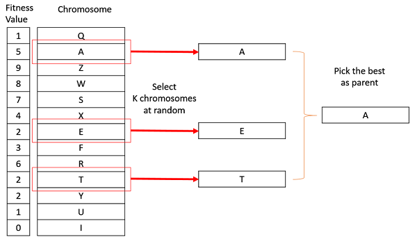
Tournament selection being performed on a population of size 13. Here, \(k = 3\), meaning three chromosomes were selected at random. Of the three, the candidate solution with the highest fitness is then returned as the selected chromosome.
The value of \(k\) is typically kept low, but can be adjusted as needed
If \(k = 1\), this would be the same as a uniform selection
If \(k = \mu\), this would be the same as always selecting the best
As \(k\) increases, so does the selection pressure
11.3. Fitness Proportional Selection
There are a collection of selection strategies that are fitness proportional
The probability of selecting an individual depends on its fitness value compared to the whole population’s fitness
The simplest of these is to have the probability be the individual’s proportion of the total population fitness
\(p(i) = \frac{f(i)}{\sum^{\mu}_{j}f(j)}\)
Where \(p(i)\) is the probability of selecting individual \(i\)
And \(f(i)\) is the fitness of individual \(i\)
Note that the sum of the probabilities must be one \(\sum^{\mu}_{j=1}p(j) = 1\)
The benefit here is that by selecting highly fit individuals, the search may produce high quality solutions quickly
However, this may cause the population to get stuck in a local maximum
Premature convergence
It is important to ensure the population stays diverse
Further, when the population begins to converge, this strategy becomes similar to a uniform selection
Learning will stagnate when the fitness values of the chromosomes within the population are similar
Modifications to this strategy include adding some constant or windowing
Windowing is subtracting the minimum fitness within the population from all individuals within the population
Several selection probabilities are shown in the below table for some maximization problem
One regular, one with adding some constant, and one and windowing
Here, adding a constant made the lowest fit individual more likely to be selected
While also making the selection probabilities more similar
With windowing, the lowest fit individual had zero probability of being selected
While also making the selection probabilities more different
\(i\) |
\(f(i)\) |
\(p(i)\) for \(f(i)\) |
\(f(i) + 10\) |
\(p(i)\) for \(f(i) + 10\) |
Windowing \(p(i)\) for \(f(i)\) |
|---|---|---|---|---|---|
A |
\(1\) |
\(0.1\) |
\(11\) |
\(0.257\) |
\(0\) |
B |
\(4\) |
\(0.4\) |
\(14\) |
\(0.350\) |
\(0.333\) |
C |
\(5\) |
\(0.5\) |
\(15\) |
\(0.375\) |
\(0.666\) |
Total |
10 |
1.0 |
40 |
1.0 |
1.0 |
11.3.1. Rank Based Selection
An alternative is to take the same idea, but rank the candidate solutions
Then, have the probability of being selected related to their rank, not their fitness value
\(i\) |
\(f(i)\) |
\(p(i)\) for \(f(i)\) |
Ranking |
\(p(i)\) for Ranking |
|---|---|---|---|---|
A |
\(1\) |
\(0.1\) |
\(0\) |
\(0\) |
B |
\(4\) |
\(0.4\) |
\(1\) |
\(0.333\) |
C |
\(5\) |
\(0.5\) |
\(2\) |
\(0.666\) |
Total |
10 |
1.0 |
1.0 |
The above table shows a simple linear ranking being used, but other more complex forms may be used
The benefit of this strategy is that, as the population converges, selection pressure will not become lower
The downside is the computational overhead of ranking each candidate solution
11.3.2. Roulette Wheel Selection
Fitness proportional selection is commonly referred to as a roulette wheel selection
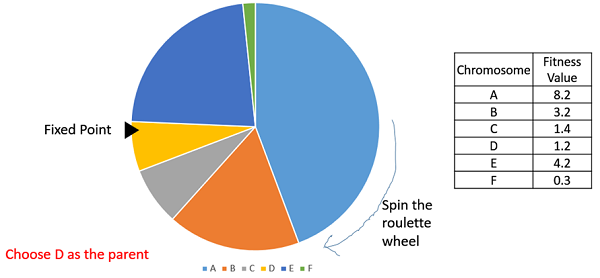
Visualization of roulette wheel selection. Each individual is assigned a piece of the wheel proportional to that individual’s proportion of fitness of the population’s total fitness.
11.3.3. Stochastic Universal Sampling
Typically, the roulette wheel has one arm and is spun \(\lambda\) times
An alternative is to spin a roulette wheel with \(\lambda\) arms once
This means the wheel is spun only once
This produces a diverse set of selected individuals
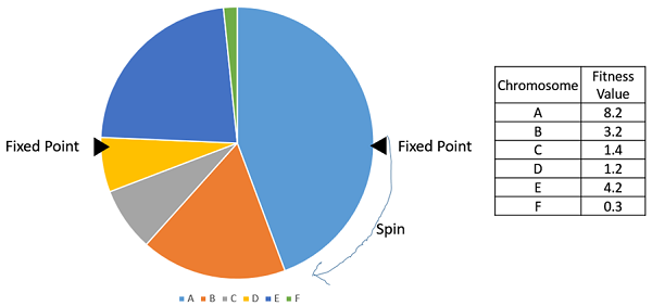
Example of a roulette wheel where \(\lambda=2\).
Warning
Although possible, fitness proportional selections often requires some alterations to work with algorithms minimizing fitness or negative fitness values.
11.4. Survivor Selection
With a steady state algorithm, survivor selection is needed
Which individuals survive and which are replaced
Any rules could be used, but common ones include
Random
Randomly select \(\lambda\) to replace
Age based
Replace the \(\lambda\) oldest individuals
Ignores fitness
Might kill off the best individuals
Fitness based
Replace the \(\lambda\) worst individuals based on fitness
Will kill off the worst candidate solutions
May cause the population to converge prematurely
Diversity based
Replace \(\lambda\) candidate solutions that are the most similar
The idea is, replace those that add little diversity to the population
Similarity based
Replace the \(\lambda\) candidate solutions with the most similar fitness to the offspring
Similar to diversity and easy to implement with an assumption
Those with a similar fitness may be similar in the genotype space
11.4.1. Elitism
Regardless of using a generational or steady state algorithm, elitism is commonly used in evolutionary computation
The idea is, always have a copy of the best \(x\) chromosomes in the population
Typically \(x=1\)
Having \(x\) too high will cause premature convergence
11.5. Diversity
Diversity is how much the members of the populations differ from one another
Diversity is important within a population
Balances exploration and exploitation
It helps to prevent premature convergence
As with anything with evolutionary computation, there are no rules on what should be done
Below are some high-level ideas, but is in no way exhaustive
Explicitly add a diversity measure to the fitness calculation
Only have similar individuals compete with one another
The Island Model
Distribute the population into sub-populations that evolve independently with periodic migrations
Ring Species
Only allow individuals to mate if they are close to one another within the population
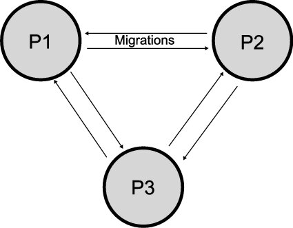
Island model layout with three sub-populations. Each of the three sub-populations evolve independently. This allows each sub-population to explore the search space along its own path, thereby preserving diversity between the sub-populations. Periodically, members of the sub-populations migrate to other sub-populations to introduce diversity to the individual sub-populations.
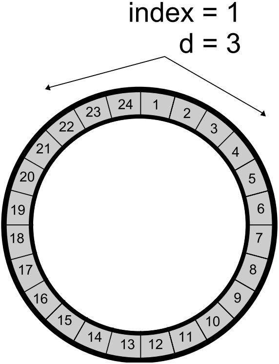
Ring species treats the population as a ring/circle and mating can only occur between chromosomes if they exist within some distance (number of indices) of one another. In this example, the distance \(d=3\), therefore only the candidate solutions at indices 22, 23, 24, 1, 2, 3, and 4 would be eligible for mating.
Further, there are no rules on where the diversity should be measured
Genotype space
How similar the chromosomes are
Depends on the encoding
Hamming distance?
Levenshtein distance?
Phenotype space
How different are the phenotypes (what the chromosomes represent)
May be very different from the genotype space’s distance
Algorithm space
Some distance based on the algorithm’s framework
For example, ring species and the island model
11.6. For Next Class
TBD