13. Symbolic Regression with Genetic Programming
The purpose of this topic is to perform symbolic regression with genetic programming
The genetic programming system being used is DEAP (Distributed Evolutionary Algorithms in Python)
Much of the heavy lifting required to implement a genetic programming algorithm is managed by DEAP
13.1. Problem — Regression Analysis
Regression is finding the relationships between dependent and independent variables given some observations
A common and simple form of regression is linear regression
Find a linear relationship between some dependent and independent variables
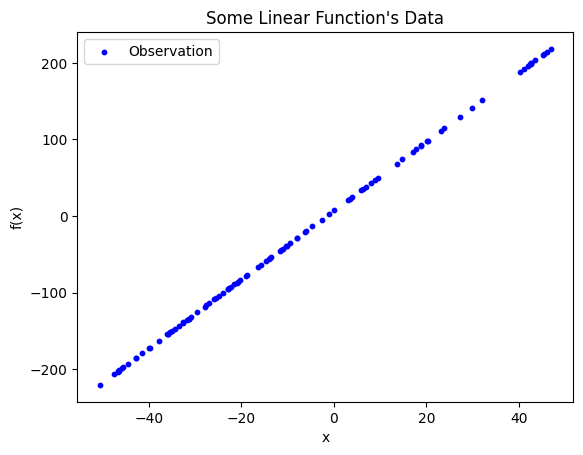
Observations of some phenomenon plotted in two dimensions. The dependent variable is plotted along the y-axis and the independent variable is along the x-axis. From a quick glance, this data clearly has some linear relationship.
Given the above observations, the goal is to draw a line of best fit
Which should look a lot like \(y = mx + b\)
The mathematics behind finding this line is interesting, but outside the scope of this course
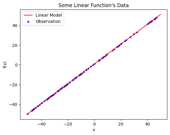
Linear model plotted on top of the observations. The resulting model is \(\hat{y} = 0.999885x + 0.997937\) and has an \(R^{2}\) value of \(0.9999885\).
The linearly regressed model for the above observations is \(\hat{y} = 0.999885x + 0.997937\)
Note that \(\hat{y}\) denotes that it is not \(y\), but only a prediction/estimation of \(y\)
This particular model has an \(R^{2}\) of \(0.9999885\)
This is a measure of goodness
The closer to 1.0, the better the fit
13.1.1. Linear Regression on Nonlinear Relationships
With linear regression, trouble arises when the observed data has nonlinear relationships
It is still possible to find a high-quality model, but it would require several assumptions and a lot of guesswork
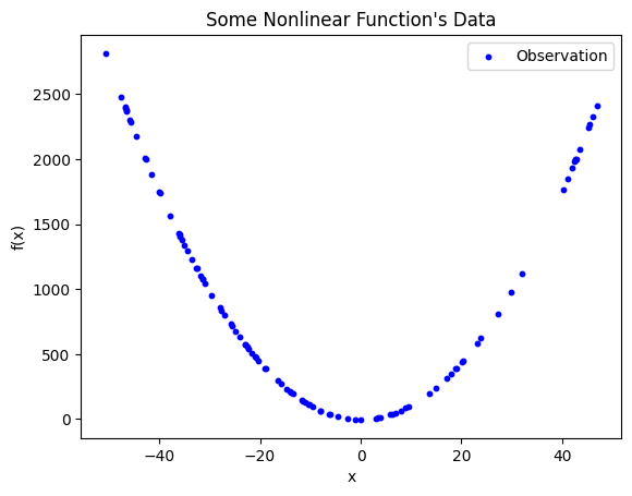
Observed data with clear nonlinear relationships. The data appears to be parabolic or hyperbolic, but may be neither depending on which segment of the function was observed. It is not possible to effectively fit a straight line to describe the relationship between the dependent and independent variable.
Nevertheless, looking for a linear model for such nonlinear data is doomed to fail
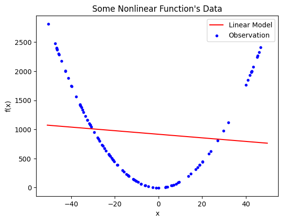
Linear model generated with linear regression on the nonlinear data. The resulting model is \(\hat{y} = -3.070395x + 916.550675\), which has an \(R^{2} = 0.010924\). Although this is the best possible straight line that fits this data, it is clear that it is not effectively fitting the data due to the limitation of the modelling strategy.
13.1.2. Symbolic Regression
An alternative strategy is something called symbolic regression
It is a form of regression analysis that requires fewer assumptions and works with nonlinear data
By using symbolic regression, the underlying nonlinear relationships may be found
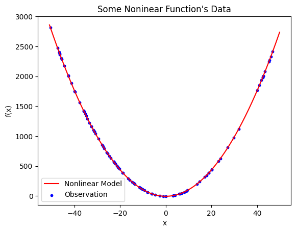
Nonlinear model found with symbolic regression. The model is \(\hat{y} = 1.100511x^{2} - 4.439578\) and has a mean squared error of \(0.162087\).
It is clear that \(\hat{y} = 1.100511x^{2} - 4.439578\) effectively describes the relationships in the data
The mean squared error is \(0.162087\)
This is not the same as \(R^{2}\)
With mean squared error, a value closer to 0.0 is better
Note
In reality, symbolic regression produced add(add(protected_divide(mul(x, x), 9.949161), mul(x, x)), -4.439578),
which was simplified to \(\hat{y} = 1.100511x^{2} - 4.439578\).
13.2. DEAP
Due to the complexity, it is not common to implement genetic programming from scratch
Instead, a genetic programming system will be used, which does much of the heavy lifting for the user
Many systems exist in various programming languages
DEAP is a framework for evolutionary computation algorithms in Python
Distributed Evolutionary Algorithms in Python — DEAP
It’s a package for implementing evolutionary computation algorithms
DEAP is not only for genetic programming, but many evolutionary computation algorithms
It includes algorithm and tools for implementing multiple types of algorithms, enhancements, and analysis
Although any genetic programming system could be used, DEAP will be used here
It is encouraged to contribute to the repository if possible
It is strongly recommended to have a look at DEAP’s documentation
13.3. Data
The data being used will be tabular
Rows of observations
Columns of variables
Below is an example of how the data would look
ARG1 (\(X_1\)) |
ARG2 (\(X_2\)) |
ARG3 (\(y\)) |
|---|---|---|
-3.16833493e+01 |
3.63253949e+01 |
-5.75550374e+02 |
-3.59771849e+01 |
1.63633781e+01 |
-2.94238014e+02 |
4.35235243e+01 |
-1.54189209e+01 |
-3.35451435e+02 |
4.19705508e+01 |
1.25491733e+01 |
2.63416737e+02 |
… |
… |
… |
For this example, the data is provided in CSV files
The data is formatted such that the last column is always the dependant variable
Thus, all proceeding columns are independent variables
This data was generated by some phenomenon
The goal is to find a model that effectively describes the relationships between the data
Loading this data can be done as follows
 98    data_file = open(os.path.join(RELATIVE_RESOURCES, DATA_FILE))
 99    all_data = [list(map(float, x.split(","))) for x in data_file]
100    independent_variables = [observation[:-1] for observation in all_data]
101    dependent_variable = [observation[-1] for observation in all_data]
The above code loads the data specified in some constants
The independent variables will be stored in a two dimensional list
Rows are observations
Columns are different independent variables
The dependent variable is stored in a one dimensional list
Each value corresponds to the independent variables at the same index
Following the example data in the above table, the values would be stored as follows
independent_variables = [[-3.16833493e+01, 3.63253949e+01],
                        [-3.59771849e+01, 1.63633781e+01],
                        [4.35235243e+01, -1.54189209e+01],
                        [4.19705508e+01, 1.25491733e+01],
                        ... ]

dependant_variable = [-5.75550374e+02, -2.94238014e+02, -3.35451435e+02, 2.63416737e+02, ...]
13.4. Evaluation
A common mechanism for evaluating genetic programming performing symbolic regression is mean squared error
\(\frac{1}{n}\sum_{i}^{n}(y_{i} - \hat{y_{i}})^{2}\)
A mean squared error of zero is perfect
Any metric could be used, but mean squared error is very popular
One of the reasons it is used is because it punishes bigger errors more
If the difference between the observed and estimated value is 1, the squared error is 1
If the difference is 2, the error is 4
If it’s 3, the error is 9
…
In other words, it’s much worse to be very wrong than it is to be a little wrong
49def mean_squared_error(
50    compiled_individual, independent_variables: list[list[float]], dependent_variable: list[float]
51) -> float:
52    """
53    Calculate the mean squared error for a given function on the observed data. The independent variables are a list of
54    lists where the list of the outer list is the number of observations and the length of the inside list is the number
55    of independent variables. The length of the dependent variables is the number of observations.
56
57    :param compiled_individual: A callable function that the dependent variables are give to as arguments
58    :param independent_variables: Values given to the function to predict
59    :param dependent_variable: Expected result of the function
60    :return: Mean squared error of the function on the observed data
61    """
62    running_error_squared_sum = 0
63    for xs, y in zip(independent_variables, dependent_variable):
64        y_hat = compiled_individual(*xs)
65        running_error_squared_sum += (y - y_hat) ** 2
66    return running_error_squared_sum / len(dependent_variable)
13.5. Language
With symbolic regression, genetic programming will be searching the space of mathematical expressions
This includes both the operators and operands
The language is the set of operators and operands that the genetic programming system can use in the search
The trouble is, it’s not always clear which operators and operands should be included
Thus, the design of the language may need to be tuned for evolution like other hyperparameters
Fortunately, with symbolic regression, there is a common set to start with
Typical arithmatic operators
Maybe some trigonometry functions
Maybe logarithm and exponentials or even natural log and Euler’s number
However, there is a potential problem with divide as the evolutionary search may try to divide by zero
For this reason, it is common to see a protected divide used instead
If attempting to divide by zero, return infinity
34def protected_divide(dividend: float, divisor: float) -> float:
35    """
36    The basic arithmetic operator of division. If the division basic results in a ZeroDivisionError, this function
37    returns an arbitrarily large number (999,999,999).
38
39    :param dividend: Value to divide
40    :param divisor: Value to divide by
41    :return: The quotient; the result of the division (dividend/divisor)
42    """
43    if divisor == 0:
44        return math.inf
45    else:
46        return dividend / divisor
Setting up the language with DEAP is then done like below
105    primitive_set = gp.PrimitiveSet("MAIN", len(independent_variables[0]))
106    primitive_set.addPrimitive(operator.add, 2)
107    primitive_set.addPrimitive(operator.sub, 2)
108    primitive_set.addPrimitive(operator.mul, 2)
109    primitive_set.addPrimitive(protected_divide, 2)
110    primitive_set.addPrimitive(operator.neg, 1)
111    primitive_set.addEphemeralConstant("rand_int", partial(randint, -10, 10))
The first line, creating the
PrimitiveSetobject, is where the language operators and operands will be addedIt also specifies the number of independent variables the function will have as the second argument
As discussed above, the independent variables are stored in some list called
independent_variables
Each operator is added to the primitive set object along with the number of operands that operator requires
The operator is the first argument, and is passed as a function
Most of the added operators in this example are taken from the
operatorlibraryThe protected divide, described above, is also added
The
negoperator is the negation (multiply by -1) and only requires one operand
Finally, the constant values are added with
addEphemeralConstantIn this example, integers between -10 and 10 are eligible
Warning
There is no guarantee or suggestion that this is a good language, but it is at least a reasonable place to start.
13.6. DEAP Setup
Below is an example of a setup for a DEAP algorithm
It effectively defines what each part of the algorithm will be
115    creator.create("FitnessMinimum", base.Fitness, weights=(-1.0,))
116    creator.create("Individual", gp.PrimitiveTree, fitness=creator.FitnessMinimum)
117
118    toolbox = base.Toolbox()
119    toolbox.register("generate_tree", gp.genHalfAndHalf, pset=primitive_set, min_=1, max_=4)
120    toolbox.register("individual", tools.initIterate, creator.Individual, toolbox.generate_tree)
121    toolbox.register("population", tools.initRepeat, list, toolbox.individual)
122    toolbox.register("compile", gp.compile, pset=primitive_set)
123    toolbox.register(
124        "evaluate",
125        mean_squared_error_fitness,
126        toolbox=toolbox,
127        independent_variables=independent_variables,
128        dependent_variable=dependent_variable,
129    )
130    toolbox.register("select", tools.selTournament, tournsize=TOURNAMENT_SIZE)
131    toolbox.register("mate", gp.cxOnePoint)
132    toolbox.register("generate_mutation_subtree", gp.genFull, min_=0, max_=4)
133    toolbox.register("mutate", gp.mutUniform, expr=toolbox.generate_mutation_subtree, pset=primitive_set)
This code
Sets the problem to be a minimization problem
Says how the individuals (chromosomes) will be encoded
Defines how the individuals and population will be generated
It defines the evaluation metric
Note that
mean_squared_error_fitnessis not the function described aboveMore on this below
It also sets the selection strategy and genetic operators
DEAP requires that the fitness function return a tuple of results
However, the above
mean_squared_errorfunction returns only a single valueThus, another function,
mean_squared_error_fitness, is created that callsmean_squared_errorThis function also
Checks if exceptions should be thrown
Compiles the trees into something that can be functionally evaluated
Wraps the mean squared error in a tuple to be returned
69def mean_squared_error_fitness(
70    individual, toolbox, independent_variables: list[list[float]], dependent_variable: list[float]
71) -> tuple[float]:
72    """
73    Calculate the mean squared error for a given function on the observed data. The independent variables are a list of
74    lists where the list of the outer list is the number of observations and the length of the inside list is the number
75    of independent variables. The length of the dependent variables is the number of observations.
76
77    :param individual: A deap representation of a function that the dependent variables are give to as arguments
78    :param toolbox: A deap toolbox
79    :param independent_variables: Values given to the function to predict
80    :param dependent_variable: Expected result of the function
81    :return: A tuple containing the mean squared error of the function on the observed data
82    :raises ValueError: If the number of observations s 0 or if there are a different number of observations
83    """
84    if len(independent_variables) == 0 or len(dependent_variable) == 0:
85        raise ValueError("Number of dependent and independent variables must be greater than 0")
86    if len(independent_variables) != len(dependent_variable):
87        raise ValueError(
88            f"Uneven number of observations of independent and dependent variables: "
89            f"{len(independent_variables)}, {len(dependent_variable)}"
90        )
91    callable_function = toolbox.compile(expr=individual)
92    individual_mean_squared_error = mean_squared_error(callable_function, independent_variables, dependent_variable)
93    return (individual_mean_squared_error,)
13.6.1. Bloat Control
As mentioned in the previous topic, genetic programming suffers from bloat
The trees tend to grow larger with no improvement in fitness
This negatively impacts the algorithm’s performance
DEAP provides simple ways to control bloat
137    toolbox.decorate("mate", gp.staticLimit(key=operator.attrgetter("height"), max_value=MAX_HEIGHT))
138    toolbox.decorate("mutate", gp.staticLimit(key=operator.attrgetter("height"), max_value=MAX_HEIGHT))
139    toolbox.decorate("mate", gp.staticLimit(key=len, max_value=MAX_NODES))
140    toolbox.decorate("mutate", gp.staticLimit(key=len, max_value=MAX_NODES))
The above sets limits on how deep and how many nodes a tree may have after a genetic operator is applied
These values may need to be adjusted to improve performance
If they are allowed to get too big, the search may take too long
If they are not allowed to get big enough, it may not be possible to model the data
13.6.2. Bookkeeping
DEAP also provides tools for keeping track of the results throughout evolution
144    hall_of_fame = tools.HallOfFame(1)
145    stats_fit = tools.Statistics(lambda individual: individual.fitness.values)
146    stats_size = tools.Statistics(len)
147    stats_height = tools.Statistics(operator.attrgetter("height"))
148    mstats = tools.MultiStatistics(fitness=stats_fit, size=stats_size, height=stats_height)
149    mstats.register("avg", numpy.mean)
150    mstats.register("std", numpy.std)
151    mstats.register("min", numpy.min)
152    mstats.register("max", numpy.max)
The above code creates a
HallOfFame, which will keep track of the top candidate solution for each generationIt also keeps track of some summary statistics on some population metrics
Population average, standard deviation, minimum, and maximum for fitness, tree height, and tree size
These values will be recorded for each generation
13.7. Running and Results
After all the setup, running the algorithm is done as follows
156    population = toolbox.population(n=POPULATION_SIZE)
157    population, log = algorithms.eaSimple(
158        population,
159        toolbox,
160        CROSSOVER_RATE,
161        MUTATION_RATE,
162        GENERATIONS,
163        stats=mstats,
164        halloffame=hall_of_fame,
165        verbose=True,
166    )
With the above settings, output like the following will be displayed
                                          fitness                                                      height                                             size
            -------------------------------------------------------------------     -------------------------------------------     -----------------------------------------------
gen nevals  avg             gen     max             min     nevals  std             avg     gen     max     min     nevals  std     avg     gen     max     min     nevals  std
0   10      3.07232e+08     0       2.98774e+09     472.225 10      8.93845e+08     2.3     0       4       1       10      1.1     10.2    0       30      2       10      9.67264
1   10      1.80136e+06     1       1.66745e+07     0.00906234      10      4.97235e+06     2.9     1       5       1       10      1.04403 9.7     1       26      2       10      7.0859
2   3       2331.57         2       13844.5         0.00906234      3       4034.1          2.8     2       3       2       3       0.4     6.7     2       12      4       3       2.75862
3   7       128527          3       1.26907e+06     0.00906234      7       380187          2.9     3       5       1       7       1.13578 6.9     3       14      2       7       3.53412

(rows 4 -- 96 omitted for brevity)

97  8       1.00691         97      1.00691         1.00691         8       0               0       97      0       0       8       0               1       97      1       1       8       0
98  8       86.9783         98      860.721         1.00691         8       257.914         0.1     98      1       0       8       0.3             1.2     98      3       1       8       0.6
99  7       1.00691         99      1.00691         1.00691         7       0               0       99      0       0       7       0               1       99      1       1       7       0
100 7       128571          100     1.2857e+06      1.00691         7       385711          0.2     100     2       0       7       0.6             1.3     100     4       1       7       0.9
Viewing the results requires converting the tree to a string
It is possible to have DEAP generate and display images of the expression trees
Unfortunately, it can be difficult to get working
Below is an example of displaying the top result after evolution is complete
170    print(str(hall_of_fame[0]))
171    print(hall_of_fame[0].fitness.values)
Below is an example result for a run of the GP
neg(neg(add(1, ARG0)))
(0.009062344161081039,)
Given that
ARG0is the only independent variable, the above can be simplified to \(y = x + 1\)The mean squared error of the model when applied to the data is roughly 0.00906
13.7.1. Funny Results
Given the stochastic nature of the search, the final result will differ every time
And since genetic programming’s only goal is to fit the data, and it does not attempt to simplify the results, some silly looking functions may be generated
Below are additional examples of generated solutions that all simplify to \(y = x + 1\)
sub(ARG0, protected_divide(ARG0, neg(ARG0)))
add(mul(protected_divide(ARG0, ARG0), protected_divide(ARG0, ARG0)), ARG0)
add(ARG0, protected_divide(ARG0, mul(7, protected_divide(ARG0, 7))))
add(-8, add(ARG0, 9))
add(mul(protected_divide(ARG0, ARG0), protected_divide(ARG0, ARG0)), mul(protected_divide(ARG0, 1), protected_divide(ARG0, ARG0)))
13.8. For Next Class
Check out the following script