7. Representation

The representation is how the problem is encoded
How exactly a problem is encoded is one of the first things to consider when using evolutionary computation
A problem can be encoded however one wants, but the choice can impact the quality of the evolutionary search
There are many different types of encodings
- Binary
- Integer
- Real value/floating point numbers
- Permutations
- Tree structures
- Finite state machines
- …
Certain forms of evolutionary computation are designed to work with certain encodings
However, given the nature of these algorithms, any encoding can be used as long as it produces the desired results

7.1. Genotype vs. Phenotype

As previously discussed
- The phenotype is a solution to a problem
- The genotype is an encoded solution to a problem

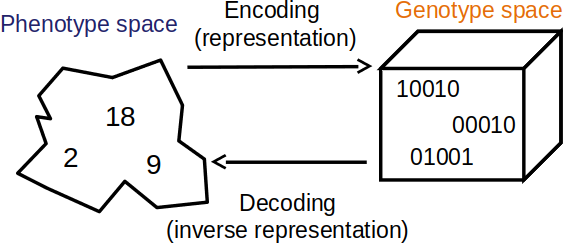
../../_images/genotype_phenotype_space.png — Visualization of the genotype and phenotype spaces. In this example, the phenotype space consists of integers while the genotype space encodes integers as unsigned binary numbers.

The choice of representation can have a large impact on the performance of the evolutionary computation algorithm
Further, the difference between solutions in the phenotype space can differ from the difference in the genotype space
- For example, consider the unsigned binary number maximization problem
- The number \(7\) is 0111 in the genotype space
- The number \(8\) is 1000 in the genotype space
- The difference in the phenotype space (\(8 - 7\)) is \(1\)
- The difference in the genotype space, if using Hamming distance, is \(4\)
  The number of bits that would need to change to get from 0111 to 1000 is \(4\)

../../_images/hamming_distance_cube.png — Graph representing the Hamming distance between the binary numbers 0 to 7. Each vertex represents a binary number and each edge between vertices represents one unit of distance. The minimum distance between vertices is the Hamming distance between the binary numbers. For example, `000` and `101` has a minimum distance of two edge between them and have a Hamming distance of two from each other.

7.1.1. TSP Example

Consider the TSP example previous discussed

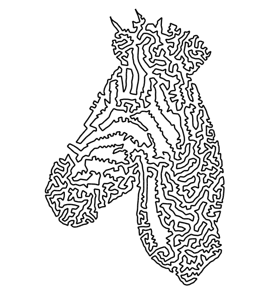
../../_images/tsp_horse.png — A solution to a large TSP instance where high-quality solutions depict a horse, or maybe a zebra? Who knows. Credit Twentylemon.

7.1.1.1. Integer Encoding

One possible encoding is an ordered list of integers representing each city
- Given \(n\) cities
- Assign each city a unique integer
- An ordered list of \(n\) integers would define a cycle
  The last city, at index \(n-1\), would return to the first city, at index \(0\)
Since the ordered list has a total of \(n\) indices
And the number of possible integers (cities) that could exist in each index is \(n\)
The search space has a size of \(n^{n}\)
- \(n\) multiplied by itself \(n\) times
Consider the following possible chromosomes
- \(<0, 0, 0, ..., 0, 0>\)
- \(<0, 0, 0, ..., 0, 1>\)
- \(<0, 0, 0, ..., 0, 2>\)
- \(...\)
- \(<0, 0, 0, ..., 0, (n-1)>\)
- \(<0, 0, 0, ..., 1, 0>\)
- \(<0, 0, 0, ..., 1, 1>\)
- \(<0, 0, 0, ..., 1, 2>\)
- \(...\)
- \(<(n-1), (n-1), (n-1), ..., (n-1)>\)
There is nothing wrong with the integer encoding
- It includes all possible Hamiltonian cycles
But the integer encoding allows inadmissible solutions to be included in the search space
For TSP, with the exception of the starting city, each city is to be visited once and only once
But with the integer encoding, it’s possible to have a chromosome where some cities are visited more than once
- Which necessarily means that some cities are not visited at all

7.1.1.2. Permutation Encoding

Given the requirement that each city is visited once and only once
- Except the starting city
The search space can be constrained such that it only includes admissible solutions
- Solutions where each city is visited once and only once
A permutation encoding where the ordered list is a permutation of the integers between \(0\) and \(n-1\)
This would ensure that each exists once and only once in the ordered list
Since the ordered list has a total of \(n\) indices
And the number of cities available for index \(0\) is \(n\)
Index \(1\) is \(n-1\)
Index \(2\) is \(n-2\)
…
Index \(n-1\) is \(1\)
The search space has size \(n!\)
This is still a very large, but it is an improvement over \(n^{n}\)

7.1.1.3. Permutation Encoding v2

The search space can be further constrained

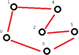
../../_images/tsp_arbitrary_path.png — Small TSP instance with some arbitrary Hamiltonian cycle shown.

In the above figure, consider the following ordered lists
- \(<0, 3, 5, 2, 4, 1>\)
- \(<2, 4, 1, 0, 3, 5>\)
Both permutations define the same Hamiltonian cycle
- In fact, there are a total of \(n\) permutations that define the exact same cycle
- This would be true for each Hamiltonian cycle
A way to eliminate the duplicates is by fixing the starting city
- Either remove it entirely from the chromosome but include it in the fitness calculation
- Or have it always at index \(0\)
This means that there only \(n-1\) remaining cities to place into the ordered list
After one is selected for visiting, there are \(n-2\) remaining cities
…
This means the search space has a size of \((n-1)!\)
This is still very large, but an improvement over \(n!\)

7.1.1.4. The Gap

The second permutation representation had a search space of \((n-1)!\)
But what is the smallest the search space could be while still including all valid solutions?

In the above figure, consider the following ordered lists
- \(<0, 3, 5, 2, 4, 1>\)
- \(<0, 1, 4, 2, 5, 3>\)
Once again, both permutations define the same Hamiltonian cycle
- The second is the reverse of the first
- For every permutation, there is a reverse of it
This means it could be possible to eliminate half of the permutations
This would result in a search space of \(\frac{(n-1)!}{2}\)
But, how could the representation be updated address this?

7.1.2. \(n\) Queens Example

Consider the \(n\) queen problem
- Place \(n\) queens on an \(n \times n\) chess board such that none can attack any other
The phenotype is the \(n \times n\) chess board configuration of \(n\) queens

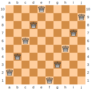
../../_images/10_queens.png — A valid configuration of \(10\) queens on a \(10 \times 10\) chess board. This particular configuration is called a “staircase solution”.

7.1.2.1. 2D Genotype

For the genotype, a 2D list encoding could be used
- It would require an \(n \times n\) list
- \(n\) cells in the list would be filled, representing the queen locations
This would be a very direct representation
- The translation from the genotype to phenotype trivial
With this encoding, there would be a search space of size \(n \times n \choose n\)
- For \(8\) queens, this is \({64 \choose 8} = 4,426,165,368\)
This search space includes all possible valid board configurations
However, it also includes a lot more invalid board configurations

7.1.2.2. 1D List of Coordinates

2D encodings can be tricky to work with
Perhaps a 1D list of \((x, y)\) coordinates would work
- It would require a list of length \(n\)
- Each value in the list would be a queen’s \((x, y)\) coordinate
This representation is a little less direct than the 2D list
- There would need to be some translation to get to the phenotype
- This is not a problem though
This encoding can also represent all possible configurations
For the size of the search space
- There are \(n\) queens to be placed
- Each queen has a \((x, y)\) coordinate
- There are \(n \times n\) possible positions for each queen
Therefore, with this encoding, the search space has a size of \((n \times n)^{n}\)
- For \(8\) queens, this is \(64^{8} = 2.815 \times 10^{14}\)
Although a 1D encoding may be easier to work with, this encoding is worse in terms of the size of the search space
- It’s worse since it’s possible for queens to be placed in the same \((x, y)\) coordinate

7.1.2.3. Integer and Permutation

Since the queens are not to attack one another, they can’t be in the same row or column
- Otherwise it will be an invalid configuration
Since each column can only have one queen in it, an integer encoding could be used
- Have a list of size \(n\)
- The index in the list corresponds to the queen’s \(x\) coordinate
- The value at the index corresponds to the queen’s \(y\) coordinate
This can be taken a step further — use a permutation representation
This would ensure that the values in each index are unique
- This would mean no two queens could be in the same row
In other words, with the permutation encoding
- Each queen must be in a different column as the columns are defined by the index of the list
- Each queen must be in a different row since the rows are defined by the values in the list, which are unique

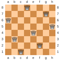
../../_images/8_queens.png — A valid configuration for the \(8\) queens problem. The permutation encoding of this solution would be \(<2, 5, 7, 0, 4, 6, 1, 3>\).

This representation eliminates all configurations where queens conflict in the rows or columns
The only way a permutation would not be a valid configuration is if any queens conflict along the diagonals
The size of the search space with this encoding is \(n!\)
- For \(8\) queens, this is \(8! = 40,320\)

Warning

The above problems are common “toy problems” that are well understood and are thus relatively easy to reason about. This enabled an intuitive process of reducing the search space by changing the representations.

Evolutionary computation, in practice, is used on difficult problems that are not well understood. Further, little may be known about the search space, it’s shape, and what all admissible and non-admissible solutions are. This means that reasoning about the representation may not be straightforward.

7.2. Common Representations

Below a collection of common encodings are discussed
- However, the representation can be whatever one needs or wants it to be
- For example, consider the 2D list encoding for \(n\) queens discussed above
Some of these encodings fit well with a particular type of evolutionary computation algorithm
Some of these encodings are effectively what defines a class of evolutionary computation algorithm

7.2.1. Binary Representation

A collection of \(0\)s and \(1\)s
- Like the representation used for the maximization of an unsigned binary number previously discussed
- For example, \(<0, 1, 1, 0, 1, 1, 1, 0, 0, 0, 0, 1>\)
Commonly used for binary decisions
Can be used to represent virtually anything as long as there is a sufficient encoding/decoding method
- This representation is often very indirect

7.2.2. Integer Representation

A collection of integers
Could be any integer or integers taken from a predefined set of integers
For example
- Allow all integers representable in Python
- Allow only \(0, 1, 2\) and \(3\) to mean North, South, East, West
The ordering of the integer values may or may not matter
- Although \(0\) comes before \(1\), North is not less than South
The order of the elements in the collection may or may not matter
- The fact that one integer is at index \(7\) and another is in index \(8\) may not matter
The encoding could be used to represent whatever, as long as there is a sufficient encoding/decoding method
Consider the problem of programming a robot to traverse a maze
The set of possible integers could be \(\{0, 1, 2, 3\}\) meaning North, South, East, and West
The robot needs to take \(10\) steps
A valid chromosome could be \(<0, 0, 0, 1, 0, 2, 3, 0, 2, 2>\)

7.2.3. Permutation Representation

An ordering of values in a set/multiset
- An arrangement of values in some sequence
Useful for situations where each value in an encoding must be unique, or have a fixed number of occurrences
For example, TSP
- Each Hamiltonian cycle is defined by a permutation of cities
Does not need to be numerical
Order of elements in the chromosome matters
Consider the problem of finding English words form a given multiset of letters
- Given the multiset of letters \(\{A, A, E, G, M, N, T\}\)
- Below is a list of possible chromosomes
  \(<A, A, E, G, M, N, T>\)
  
  \(<G, A, T, E, M, A, N>\)
  
  \(<M, A, G, E, N, T, A>\)
  
  \(<M, A, G, N, A, T, E>\)
  
  \(<N, A, M, E, T, A, G>\)

7.2.4. Real Value Representation

A collection of real/floating point numbers
Consider the problem of encoding the weights for an artificial neural network
Or finding the \((x, y)\) coordinates to find the minimum value of some function

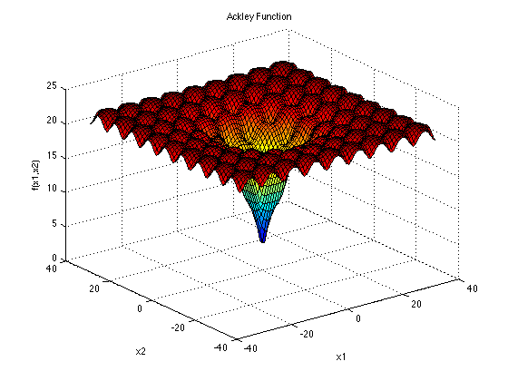
../../_images/ackley_function.png — Ackley function shown in 3D where the plotted value is the result of the function. This function is a common “toy problem” used to test optimization algorithms that work with real numbers [1].

Certain forms of evolutionary computation work well with real/floating point numbers
- Evolutionary strategies, differential evolution, and particle swarm optimization work well with real numbers

7.2.5. Tree Representation

Tree representations are typically used in genetic programming
The tree representation is used to encode a program/function

../../_images/tree_examples.png — Example of three different tree encodings for three different problems. The left tree encodes some mathematical expression, the centre tree encodes a boolean expression, and the right tree is some conditional program.

The above figure shows three different tree encodings that would be used for different problems
The left most tree represents the mathematical expression \((1.2 - x) \times y\)
- This could be used for a regression problem
The centre tree represents the boolean expression length < 5.2 or not(red)
- This could be used for programming a classifier
The right most tree represents the conditional program if(open and right closed) then (forward) else (turn right)
- This could be used for programming a robot to traverse a maze
The trees are made up of operators and operands
- Operands are the leaves of the trees and can be a variable or constant
- Operators are interior nodes and act on the values returned by their children
Many of the common representations for evolutionary computation have a fixed size
However, tree so not, and they can have odd shapes

7.3. For Next Class

TBD