10. Genetic Operators
Below is a collection of common genetic operators for broad types of representations
This is by no means exhaustive
Further, it should not be assumed that they are particularly effective
They are intended to provide foundational ideas
These operators focus on representations for genetic algorithms
The motivation for focusing on genetic algorithms is they are quite a general form of evolutionary computation
Although common genetic operators are presented, being creative and trying to invent new operators is encouraged
10.1. Genetic Operators for Binary Representations
Binary representations are those that only contain two values, which are typically 0s and 1s
10.1.1. Crossovers
10.1.1.1. One Point Crossover
Randomly select an index
Exchange the elements between the chromosomes after that index
This crossover is not particularly destructive
The amount in which the information within the chromosomes gets changed is low
This crossover works well when element adjacency in the chromosome is important
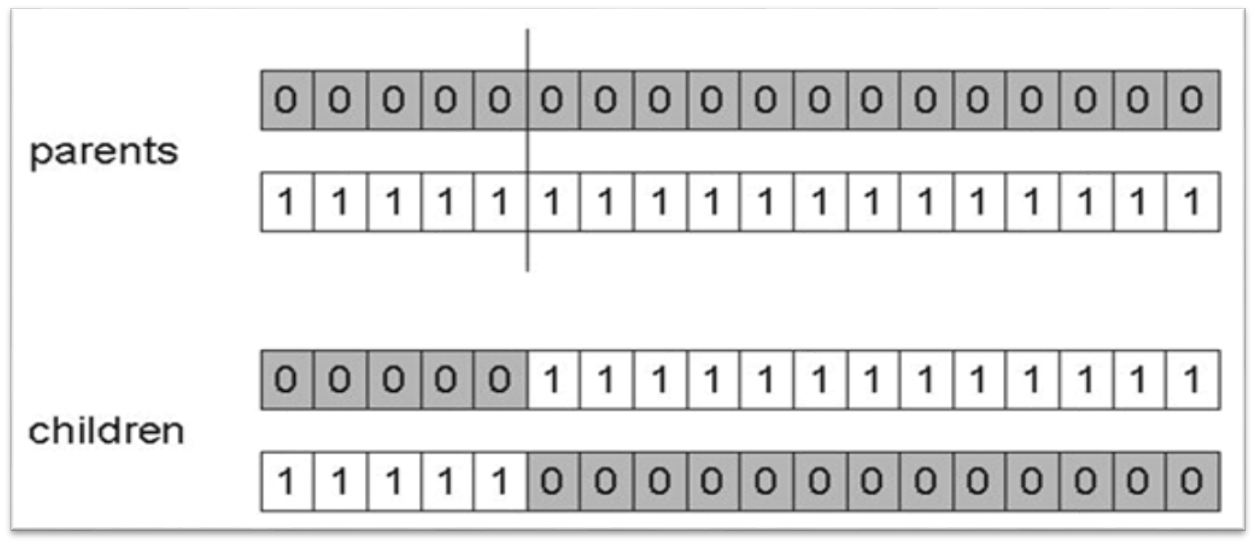
Result of applying one point crossover on two chromosomes. This example has index 5 as the randomly selected crossover point, thus, all elements after index 5 are exchanged between the parent chromosomes. Although this example shows one parent containing only 0s and the other containing only 1s, this is not a requirement; the parents could contain both 0s and 1s.
10.1.1.2. \(n\) Point Crossover
Randomly select \(n\) indices
Exchange the elements between every other pair of indices the indices
If an odd number of indices, exchange the elements from the last index to the end
This is a generalization of one point crossover
\(n=2\) is popular (two point crossover)
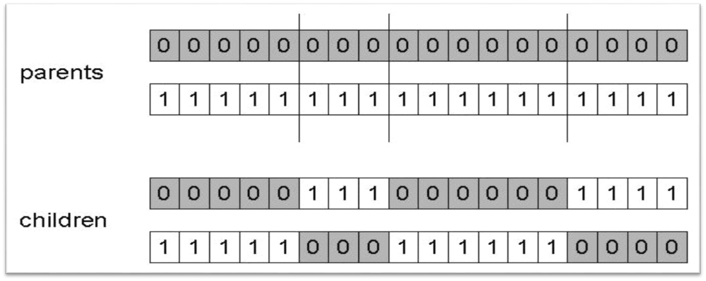
Result of applying \(n\) point crossover where \(n=3\). The randomly selected indices in this example are 5, 8, and 14. All elements between indices 5 and 8 (exclusively) are exchanged along with all the elements from index 14 to the end of the chromosome.
10.1.1.3. Uniform Crossover
Select some random number of indices at random
Exchange the elements at those indices
Often implemented by giving each index a 50/50 chance to be selected for crossover
This crossover is relatively destructive
Not particularly effective on chromosomes where element adjacency is important
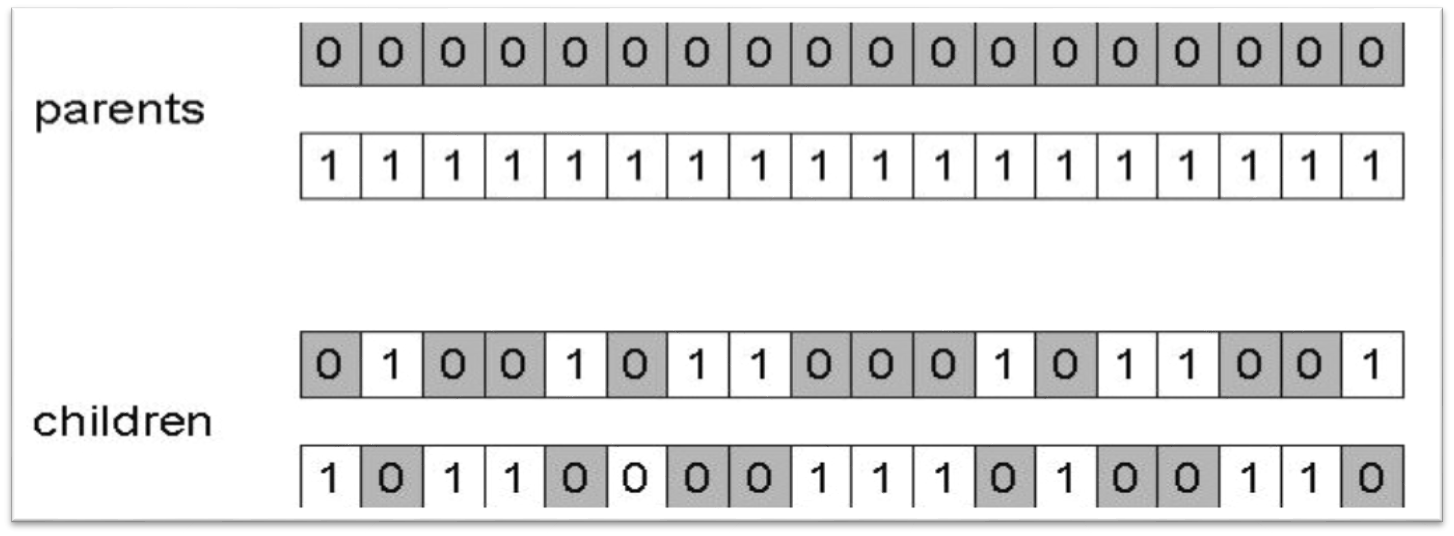
Result of applying uniform crossover where the a total of 8 values were exchanged.
10.1.2. Mutations
10.1.2.1. Bit Flip Mutation
Select some number of bits and flip them
Change 0s to 1s and 1s to 0s
The number of bits that get flipped is arbitrary
Could be hard coded
Could be randomly selected each time
Similar to uniform crossover, but instead of exchanging elements between parents, just change the binary symbol
As the number of bits that are flipped increases, so does the level of destruction this mutation causes

Result of applying a bit flip mutation to some chromosome. Here, a total of 10 bits were flipped during the mutation, which is a rather high number of bits to flip. Although this example shows the parent chromosome containing only 1s, this is not a requirement; it could have contained 0s that got changed to 1s.
10.2. Genetic Operators for Integer Representations
Integer representations are those that consist of integer values
10.2.1. Crossover
The crossovers used for binary representations are typically also used for integer representations
10.2.2. Mutations
10.2.2.1. Single Point Mutation
Sometimes called “Random Resetting”
Similar to the bit flip mutation
Select an index at random
Replace the value at the selected index with some other valid integer
A single point mutation can be generalized to an \(n\) point mutation by selecting multiple indices to change
This mutation is helpful in situations where the values within the chromosome represent cardinal attributes
Where the order of the possible integer values do not necessary matter
For example, the amount of values within a set
This mutation is also helpful in situations where each possible integer is equally likely to be within the chromosome
10.2.2.2. Swap Mutation
Select two indices at random
Swap the values at the selected indices
Can be generalized to a rotation mutation where many indices are selected and the values are rotated among them
This mutation preserves what information is within the chromosome
Now new information is added

Swap mutation applied to a chromosome where the selected indices are 1 and 4. The values at index 1 and 4 are swapped.
10.2.2.3. Creep Mutation
Select an index at random
Change the value at that index to one relatively close to the current value
For example, if the value at the selected index is 7, replace it with an 8
What close to means will depend on the context
This mutation is often used in situations where the values within the chromosome represent ordinal attributes
Where the order of the possible integer values matter
10.3. Genetic Operators for Permutation Representations
Permutation representations are those that consist of different orderings of values from some predefined set/multiset
For example
The representation used for the \(n\) queens problem was a permutation representation
Typically a permutation representation is used for TSP
Many of the previously discussed genetic operators are problematic since they may destroy the permutation property
10.3.1. Crossovers
10.3.1.1. Order Crossover
Select two indices randomly
Copy the elements between the selected indices to a child
Copy the missing elements in the child from the other chromosome in the order they appear after the second index
Best described with an example
Select two indices at random
Here, indices 3 and 7 are selected
Copy the elements between the selected indices to a child chromosome
Typically the larger index is not included in the copy
Here, elements at indices 3, 4, 5, and 6 are copied

Copy the elements between the selected indices to a child. Only one child chromosome is shown here.
Copy missing elements from the other parent to the child in the order they appear, starting at the larger index
Wrap to index 0 where necessary
Here, the copying would start at index 7, which contains the element 1
The 1 would be copied to the child as it is not contained within the child chromosome
The value at index 8 is a 4, but would not get copied since it already exists in the child
The next index would be 0 as there is no index 9, which contains a 9, thus it is copied to the child
etc.
The values that are copied are 1, 9, 3, 8, and 2, in that order

Copy the elements from the other parent, in order, starting after the larger index. Only copy values that are not already contained within the child.
Repeat the same idea for the other child
10.3.1.2. Partially Mapped Crossover
This one is rather complex and is tough to explain in words
Below are figures that help explain the process
Select two indices at random
Here, indices 3 and 7 are selected
Copy the elements between the selected indices to a child chromosome
Typically the larger index is not included in the copy
Here, elements at indices 3, 4, 5, and 6 are copied

Copy the elements between the selected indices to a child. Only one child chromosome is shown here.
Starting at the first selected index and value in the other parent, copy non-copied elements to the child by
Find the index of the element that exists in the child in the non-copied parent
Here, the value of 8 is at index 3 in the non-copied parent and is also not in the child
The value in index 3 of the child is 4
The value of 4 exists at index 8 in the non-copied parent
Thus, the value of 8 is placed into index 8
It is possible that the index the value should be copied to is already filled
See the value 2 in the below figure
The value 2 would be copied to index 6, but index 6 is already occupied in the child chromosome
When this happens, the process is continued by looking back to what value exists at that index in the child

Example of how the values of 8 and 2 would be copied to the child.
Copy the remaining elements to the child in place

The elements that do not exist in the child are copied from the parent in place.
10.3.1.3. Cycle Crossover
Select an index at random
Identify the value at that index in parent 1
Get the value at the selected index in parent 2
Find the index of that value in parent 1
Repeat until a whole cycle is found
When the value at the original index in parent 1 is found in parent 2
Exchange the elements at the indices in the cycle between the parents

Three different cycles in the same two parents. One is shown in dark grey, one in white, and one in light grey. If the light grey cycle was selected (the one only containing 6s), no change would happen as a result of this crossover.

Result of applying cycle crossover. This is the result of using either the dark grey or white cycles identified above.
10.3.2. Mutations
The swap mutation discussed above is simple and works well
Same with the generalized rotation mutation
10.3.2.1. Insertion Mutation
Select two indices at random
Insert/move the value at one index before/after the value at the other index

Result of applying insertion mutation on a chromosome where indices 1 and 4 are selected. The value at index 4 was inserted after the value at index 1.
10.3.2.2. Scramble Mutation
Select two indices at random
Scramble/shuffle the vales between the selected indices
This mutation can be quite destructive

Scramble mutation being applied between indices 1 and 5 (exclusive). The resulting order of the shown scramble is arbitrary.
10.3.2.3. Inversion Mutation
Select two indices at random
Reverse the order of the elements between the selected indices
Not particularly destructive when the adjacency of elements in the chromosome is important

Inversion mutation applied to a chromosome where the selected indices are 1 and 5 (exclusive).
10.4. Genetic Operators for Floating Point/Real Number Representations
Floating point/real number representations are those that consist of continuous values
They are bound by the computer’s ability to represent real numbers as floating point numbers
There are many complex genetic operators for floating point/real number representations
Only a few of the relatively simple popular ones are discussed here
In practice, there are other forms of evolutionary computation that perform better with these representations
10.4.1. Crossovers
Two broad ideas
Discrete — offspring have values from parents
These would be those that were discussed for the binary representation
Intermediate — offing have values between the two parents
Select intermediate crossovers are discussed below
10.4.1.1. Single Arithmetic Crossover
Randomly select an index
Average the values between the parents at that index

Result of single arithmetic crossover where the selected index was 7. The values of 0.8 and 0.2 in the two parents are replaced with 0.5, the average of the values.
10.4.1.2. Simple Arithmetic Crossover
Similar to single point crossover
Randomly select an index
Average the values between the parents after that index
This crossover can be generalized to an \(n\) point version

Result of simple arithmetic crossover where the selected index was 6. All values are averaged between the parents from index 6 to the end.
10.4.1.3. Whole Arithmetic Crossover
Average the values between the parents across all indices
This would be a special case of simple arithmetic crossover where the selected index was 0

Result of whole arithmetic crossover. All values are averaged between the parents.
10.4.2. Mutations
10.4.2.1. Uniform Mutation
Randomly select an index
Replace the value at the selected index by a value from a continuous uniform distribution within some range
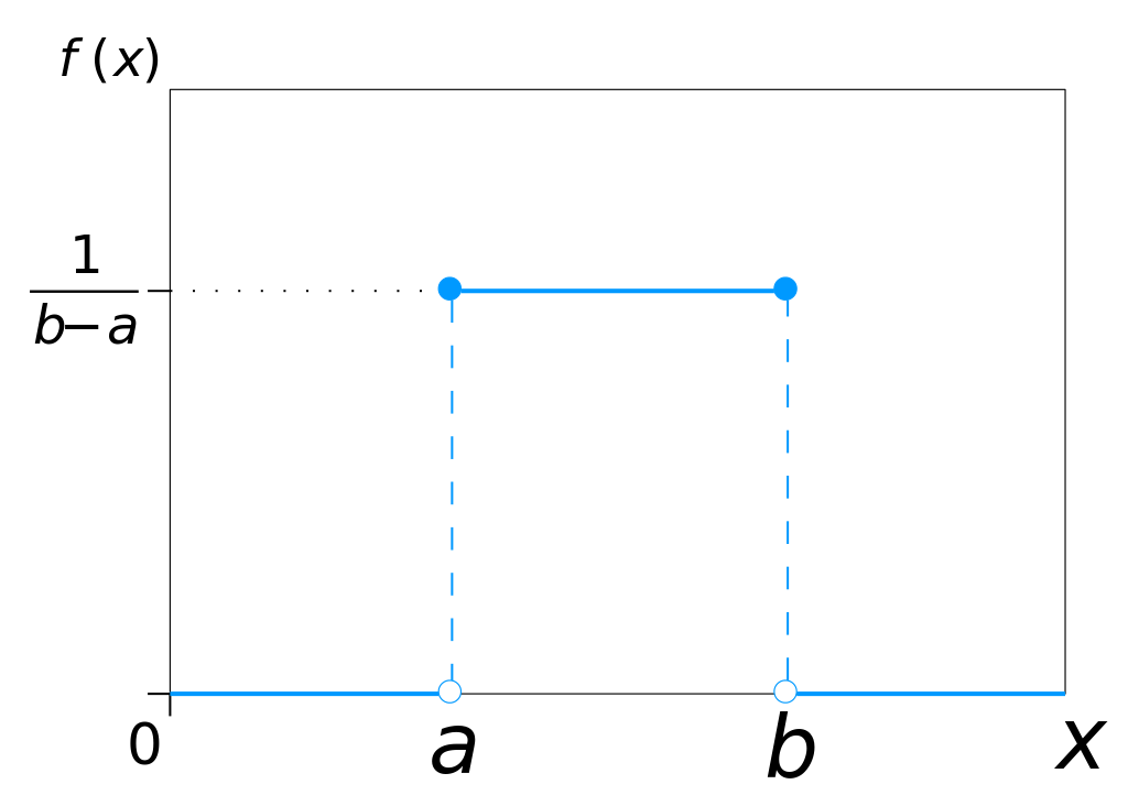
A continuous uniform distribution of values between \(a\) and \(b\).
10.4.2.2. Gaussian Mutation
Sometimes called non uniform mutation
Randomly select an index
Replace the value at the selected index by a value from a continuous normal/Gaussian distribution
The mean of the distribution is the original value at the selected index
This mutation is more likely to make small incremental changes
This mutation is particularly popular
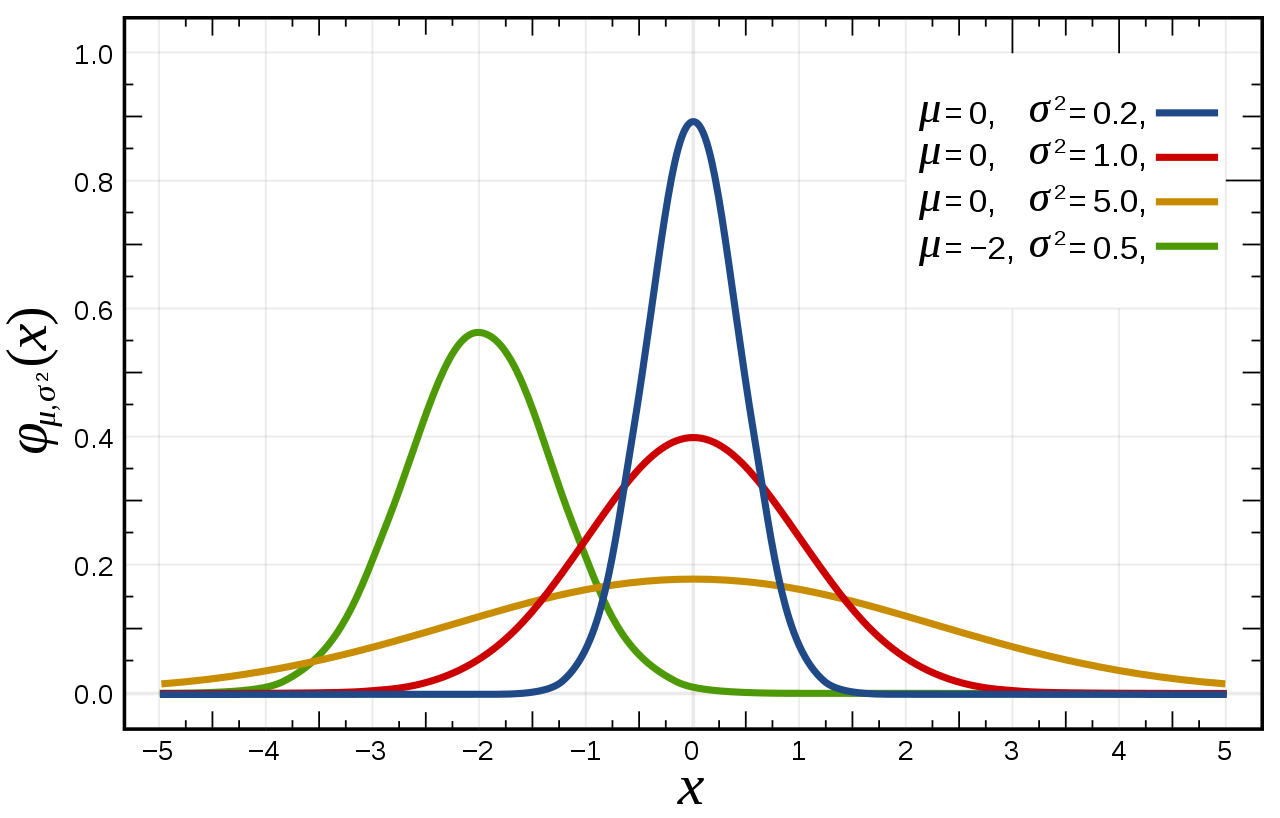
Three continuous normal/Gaussian distribution of values with different mean and variance values. The red curve is a “standard” normal distribution — has a mean of 0 and a standard deviation of 1.
10.4.2.3. Self Adapted Mutation
A non uniform mutation, but the value of the variance of the normal/Gaussian distribution is part of the chromosome
The value of the variance is also evolved
This means the evolutionary search is also modifying the value of one of it’s parameters
10.5. Genetic Operators for Tree Representations
Tree representations are typically for genetic programming
However, genetic programming is really just a genetic algorithm where
The representation is a tree
The goal is to evolve some function/program
The generic operators can become tricky when working with typed genetic programming
This is discussed in a future topic
10.5.1. Crossover
Randomly select a node within each tree
Swap the subtrees between the parents
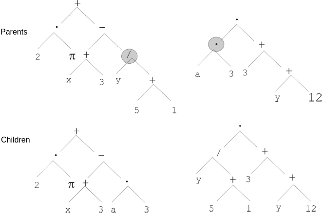
Swapping the subtrees rooted at the divide (\(/\)) and multiplication (\(\cdot\)).
10.5.2. Mutation
Randomly select a node within the tree
Replace the subtree at that node with a newly generated subtree
Typically the newly generated subtree will be of some bound depth
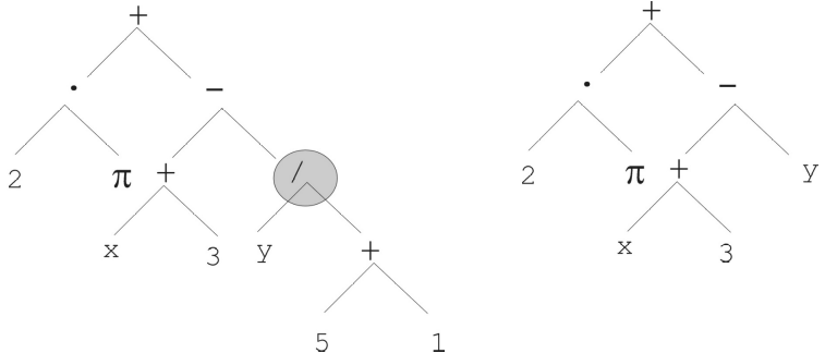
The subtree with the root of divide (\(/\)) is replaced by the subtree of only the variable \(y\). Although the subtree is replaced with a new tree with only a root node, this is not a requirement.
10.6. Additional Notes
As stated above, this list is in no way exhaustive
It simply contains some common examples of genetic operators for various representations
The above are shown to give an idea of what is out there and what works
However, throughout this course, being creative and inventive with genetic operators is strongly encouraged
10.6.1. Destructive Operators
The word destructive was used above when referring to genetic operators
This term is not particularly well defined
Used to communicate how much the chromosomes change and/or how much the information within the chromosomes change
How destructive something is will depend on the representation and the problem
For example, a single point crossover on an integer representation for a robot navigating a maze
On average it changes half the chromosome, but the information in the chromosomes is preserved and transferred
The part of the chromosome that is transferred represents a sub-path that will move to the other chromosome
This is not particularly destructive
On the other hand, a uniform crossover on the same problem can be quite destructive
Since the integer adjacent is important for paths, changing out multiple single directions can have a large impact
10.6.2. Exploration vs. Exploitation
Consider the following population for a genetic algorithm maximizing the integer value with a single point crossover
This example was already discussed in an earlier topic
[[1, 0, 1, 1, 1],
 [1, 0, 0, 0, 1],
 [0, 0, 1, 1, 1],
 [1, 0, 1, 1, 1],
 [0, 0, 0, 1, 0]]
Notice how there exists no
1in any of the chromosomes’ index 1No matter how much the search exploits the information in the population, it cannot possibly add a
1to index 1Exploit in this context means making use of what is already known to be good
Because of this, it is not possible to find the optimal solution with single point crossover alone
This is where the bit flip mutation came in
It added new information to the population; it explored the search space
In this context, the bit flip was relatively destructive compared to the one point crossover
Thus, sometimes a destructive operator is very beneficial
It can improve the search’s ability to explore other areas of the search space
Further, consider a population that has converged on some local optimum
No matter how much the information in the local optimum is exploited, the search will likely remain stuck
By increasing the exploration, perhaps the search can work itself out of the local optimum
Note
These ideas are just high-level guidelines. Crossover is not always exploitative, nor is mutation always explorative. A destructive genetic operator is not always explorative nor is a less destructive one more exploitative.
These all depend on the context of the problem, representation, and how the operators are being used. In other words, use these ideas as a starting point for high-level decision making.
10.7. For Next Class
TBD