4. Problems
The maximization of the decimal integer value of an unsigned binary number was a toy problem
It is a trivial problem that, in practice, one would not use evolutionary computation for
Evolutionary computation is typically used for problems with no known reasonable approach to address
It’s a strategy to be used as a last resort
It is computationally expensive
It’s often harder to understand compared to other algorithms
Depending on the problem, it is notorious for overfitting
For learning purposes, classic toy problems will be used in this course
But it is important to know which types of problems evolutionary computation is appropriate for
4.1. Systems
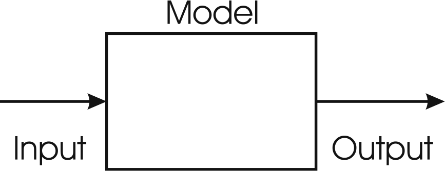
Abstract representation of a general system. Systems typically receive some input, perform some function, and produce some form of output.
Above is a simple black-box representation is a system
The system receives some number of inputs
The system performs some operation on the input
The system produces some form of output
Thinking of a system in this way helps distinguish the three important components
For concrete examples, consider
Calculating a grocery bill
Input — Prices of the items being purchased
Model — Sum the prices plus a sales tax calculation
Output — A grocery bill
Designing an aircraft wing
Input — Shape of the wing
Model — Equations of complex fluid dynamics
Output — Estimates of drag and lift
Photosynthesis
Input — Light, carbon dioxide, and water
Model — Light reactions and the Calvin cycle
Output — Oxygen and sugar
Calculating the time it takes to drive to work
Input — Route taken
Model — Spacetime
Output — Time taken
As computer scientists, we often like to think of the model as some function
Take some real world thing (in vivo) and try to model it with a computer (in silico)
With a known model, the output can be computer for any valid input
4.2. Optimization

Given a system, if the goal is to find the best set of inputs, then it is called an optimization problem.
Optimization takes place when the model and output objectives are known, but the input is not
The search space is the set of all possible inputs
For example, finding the path to work that results in the smallest amount of time possible
The search space would be all possible paths to work
Though, most of the paths would be terrible, so it is common to constrain the search space
For example, assuming living and working in the same town, do not consider paths that go out of town
4.2.1. Travelling Salesman Problem
The Travelling Salesman Problem (TSP) is a classic optimization problem
TSP can be modelled as an undirected weighted graph, such that cities are the graph’s vertices, paths are the graph’s edges, and a path’s distance is the edge’s weight. It is a minimization problem starting and finishing at a specified vertex after having visited each other vertex exactly once [1].
Effectively, the problem is to find the shortest Hamiltonian cycle within the graph

Example of a small TSP instance with four cities (vertices). In this example, each city has a path (edge) to all other cities that has an associated weight.
To think of this in terms of the three parts of a system
Given a Hamiltonian cycle (input)
Sum the edges of the weights in the cycle (model)
Return the total cycle length (output)
But this is just a description of the system, not the description of an optimization problem
To frame this as an optimization problem, find the Hamiltonian cycle that produces the smallest possible cycle length
There is a trivial algorithm to solve any instance of this problem
Find the length of all possible Hamiltonian cycles
Pick the path with the smallest cycle length
Given a set of vertices \(V\), the computational complexity of calculating a cycle length is \(O(|V|)\)
Thus, it’s only a matter of applying a linear time algorithm to each cycle
4.2.1.1. How Many Cycles are There?
The starting/ending city is always fixed
Given the four city example above and a set starting city, how many cities are there that could be visited next?
\(3\)
After the next city is picked, how many possible cities are there to visit next?
\(2\)
After that, there is only \(1\) city remaining
Therefore, there should be a total of 6 possible cycles (\(3 \times 2 \times 1 = (4 - 1)!\))
\(A \rightarrow B \rightarrow C \rightarrow D \rightarrow A\)
\(A \rightarrow B \rightarrow D \rightarrow C \rightarrow A\)
\(A \rightarrow C \rightarrow B \rightarrow D \rightarrow A\)
\(A \rightarrow D \rightarrow C \rightarrow B \rightarrow A\)
\(A \rightarrow C \rightarrow D \rightarrow B \rightarrow A\)
\(A \rightarrow D \rightarrow B \rightarrow C \rightarrow A\)
Half of these cycles are just the reverse of another cycles, so they can be ignored
To generalize this, the number of possible cycles is \(\frac{(|V|-1)!}{2}\)
How many possible cycles are there for an instance of \(100\) cities then?
\(\frac{(100-1)!}{2} = \frac{99!}{2} = 4.666311\times10^{155}\)
For a point of reference, there are about \(2.4\times10^{67}\) atoms in the Milky Way
4.2.2. \(n\) Queens
Place \(n\) queens on an \(n \times n\) chess board such that no two queens can attack each other
No two queens share the same row, column, or diagonal

Example of a backtracking algorithm searching for an admissible solution to the 8 queens problem. The 8 queens problem is a specific case of the \(n\) queens problem.
Unlike TSP, this problem is a little different for optimization
There is nothing being minimized
Instead, all that is needed is a valid board configuration
It’s binary — valid or not
4.2.2.1. How Many Board Configurations are There?
How many configurations of \(8\) queens are there on an \(8 \times 8\) board?
\(64\) choose \(8\)
\({64 \choose 8} = 4,426,165,368\)
However, there are only \(92\) valid board configurations
To generalize this, it would be \(n \times n \choose n\)
4.2.3. NASA’s Problems

Image of a truss structure in space. Versions of this structure were designed with a GA to enhance vibration isolation characteristics.
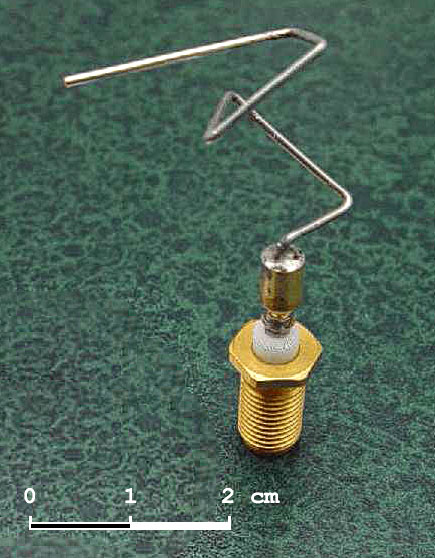
NASA’s ST5 spacecraft Antenna designed with evolutionary computation. This design maximizes the radiation pattern.
4.3. Modelling

Given a system, if the goal is to define the functionality and processes to produce the output, then it is called modelling.
Writing software is modelling
Sometimes it’s a simple problem, like writing a program to calculate a grocery bill
But sometimes it’s complex, like writing a classifier for iris classification based on petal and sepal sizes

Example iris flowers. Iris classification is a classic toy machine learning problem
When using machine learning and AI for modelling, one can think of this modelling as an optimization problem
Find the best classifier setup
For example, find a classifier (model) to classify the irises (input) such that the error (output) is minimized
The search space is the set of all possible models
4.3.1. Real World Problem
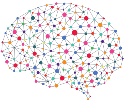
Find a model that best describes the relationships between regions of interest within a human brain during some task.
4.4. Simulation

Given a system, if the goal is to know the output of applying some input to a model, then it is called simulation.
Simulation occurs when the input and model is known, but the output is not known
Simulation is used when real world experiments may not be feasible
4.5. Search Problems
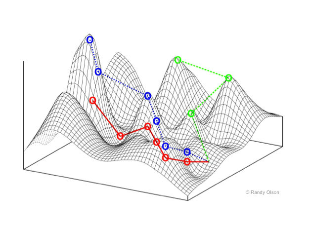
Example search space, or, fitness landscape. This example has two dimensions plus the z-dimension representing fitness. As the location in 2D space changes, the fitness value changes.
If the search space is small enough, then it may be possible to enumerate all possible configurations
However, the search space can be enormous, or even infinite
When framing problems as a search problem, one can think of the problem solver as a mechanism to traverse that space
For example, a GA traversing the search space of all possible Hamiltonian cycles for a TSP instance
It also allows for asking questions like
What is a good way to traverse the space?
Can the search be changed?
Can a feature of the search space be exploited?
Can the space be constrained or simplified?
4.6. Optimization vs Constraints
Objective functions (fitness functions in the context of evolutionary computation) are used for optimization
With TSP, minimize the total distance of the Hamiltonian cycle
A binary evaluation checks if a given constraint holds
With \(n\)-queens, are all queens safe?
Sometimes optimization problems have constraints
Consider TSP with a requirement that some city \(X\) is visited before city \(Y\)
It is also sometimes possible to convert constraint problems
Instead of finding a chess board configuration with no attacking queens, minimize the number of attacking queens
Further, it is sometimes possible to add constrains to an optimization problem to reduce the size of the search space
Like in the example above — not looking for paths to work that go out of town
4.7. Hardness
For simplicity
A problem is easy if there is some fast solver for it
A problem is hard if there is no fast solver for it
4.7.1. Continuous vs Discrete
If the problem is defined in terms of continuous values (like real numbers), it is called numerical optimization
These problems have uncountably infinite search spaces
If the problem is defined in terms of discrete values (like integers), then it is called combinatorial optimization
These problems have finite or countably infinite search spaces
4.7.2. What to Know About Hardness
Class P are decision problems that can be solved in polynomial time
Class NP are decision problems with positive solutions that can be verified in polynomial time
For example, restricted subset sum — does there exist a subset of a set of integers that sums to \(0\)?
Class P \(\subseteq\) Class NP
Class NP-Complete are decision problems with no known polynomial time algorithm but can be verified in polynomial time
All NP-Complete problems are reducible to one another
Class NP-Hard are decision problems with no known polynomial time algorithm and can’t be verified in polynomial time
For example, the decision version of TSP

Relationships between P, NP, NP-Complete, and NP-Hard class problems. Both assumptions of P \(\ne\) NP and P \(=\) NP are included.
4.7.3. What to Really Know about Hardness
There are some very hard problems out there
Given this, the goal is often to find a good enough solution to these hard problems
This is where tools like evolutionary computation comes in
4.8. For Next Class
TBD