16. What Comparing Distributions Means
Given two evolutionary computation instances, how does one determine which is better?
16.1. Random Variables
Warning
The content within this topic is kept at a high level and deliberately skips some formalisms and rigor. For the purpose of this course, the level of detail provided should be sufficient.
Consider a random variable as some phenomenon that can be observed
When observing the random variable, some quantitative measurement can be taken
The time it takes to recover from the flu
The amount of nuts a squirrel buries a day
The number of people with blond hair that walk by this building between 10am – 11am on Tuesdays
The best fitness value of a genetic algorithm run
Whatever the measurement is, they can be recorded and represented as distributions
Consider the following two random variables
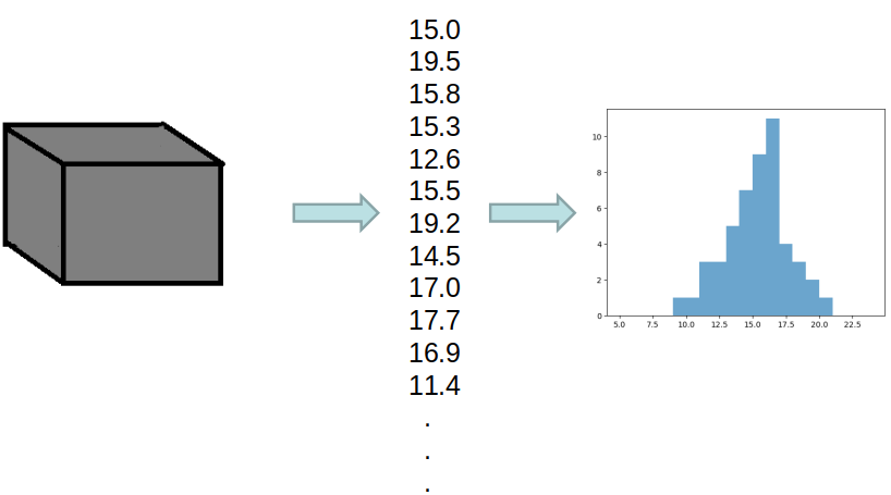
Output of some random variable represented as a box. The data is shown as a list of numbers and as a distribution. A total of 50 data points were observed and recorded.
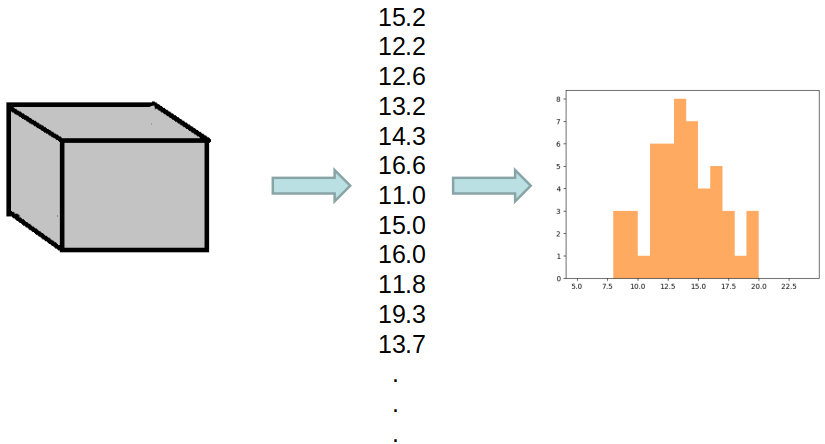
Output of another random variable represented as a box. The data is shown as a list of numbers and as a distribution. A total of 50 data points were observed and recorded.
Regardless of what these random variables are, one may wonder, are these random variables actually different?
If considering the flu recovery time
The random variables may be recovery times of two different groups of people
Does one group recover faster?
With the squirrels, does one squirrel bury more nuts in a day than the other?
Does one year have more blond people walking past the building on Tuesdays from 10am – 11am?
Does one evolutionary computation algorithm implementation perform better than another?
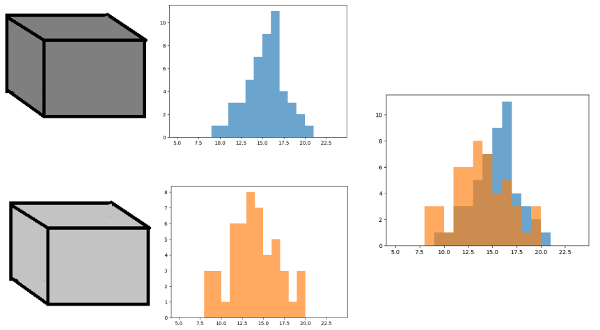
The two random variables’ measurements plotted against each other.
When visually analyzing the above comparison of the two random variables, there does appear to be a difference
But the data is clearly noisy
A range of values are obtained for each random variable
And there are only 50 observations of each random variable
It is difficult to say if these random variables are truly producing different distributions
They may effectively be the same
The two groups do not take different amounts of time to recover from the flu
The squirrel I named Jimbo does not actually bury more nuts than the squirrel I named Sir Lora
There really isn’t more blond people this year vs. last
My algorithm isn’t really performing better than the next persons’
16.2. Example — Drug Trial
Consider a drug trial
A group of 50 people is given a new drug that is intended to reduce the recovery time of the flu
Another group is given a placebo
No one in either group knows if they are given the new drug or the placebo
Here, the random variables are the two groups and the observations are the recovery times of the people in each group
Further, the recovery time is itself a random variable
This is the property/characteristic trying to be understood
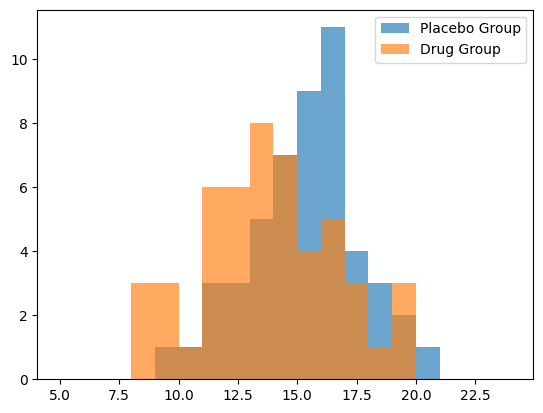
Distributions of group recovery times for individuals in the placebo group and drug group.
With the above example
The average recovery time for the placebo group was roughly 15.4 days
The average recovery time for the drug group was roughly 13.8 days
The drug group recovered, on average, 1.6 days faster
One may be tempted to conclude that the drug clearly works
However, the average recovery time is a summary statistic of a distribution
When observing the distributions, it is clear that there is more nuance
Additionally, there were only 50 observations from each group
Every individual is different and every observation is different
If I were to do this again, the distributions would look different
What are the odds that this result just happened by chance?
16.2.1. Null Hypothesis
Always start by assuming that there is no real difference
This is called the Null Hypothesis
It may feel like an arbitrary position to take, but with this assumption, it allows one to start to form an argument
Assume the drug has no actual impact on the recovery time
If the drug has no impact, then it could be expected that the average recovery time would be no different than the placebo
If both groups had the placebo, it really would not have mattered which person was assigned to which group
Thus, it should be possible to assign each individual and their corresponding recovery time to one of the two groups randomly
Therefore, the difference in the average recovery times between the two randomly assigned groups would be an example of what one would get by dumb luck
16.2.2. Permutation/Randomization Test
Assuming the null hypothesis
Shuffling the groups once and calculating the difference between the group averages will give one example of a chance difference
It is possible to generate all possible combinations of assigning the 100 people to two groups
If all possible combinations are generated, all possible average by chance differences can be calculated
Although, in this example, there are a lot
A total of \(1.01 \times 10^{29}\) combinations of splitting 100 people into two groups of 50
In cases where it is intractable to generate all combinations, simply generate some large number of combinations
Here, \(1,000,000\) combinations will be generated
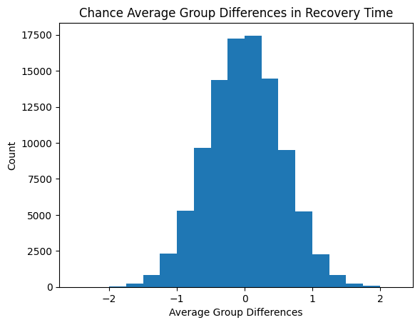
Distribution of the “by chance” average group differences after 1,000,000 shuffles of the two groups. This distribution is not the recovery times like in the above distributions.
16.2.3. Interpreting Results
The key question to ask now is, how likely is it that the original observation actually happened by chance?
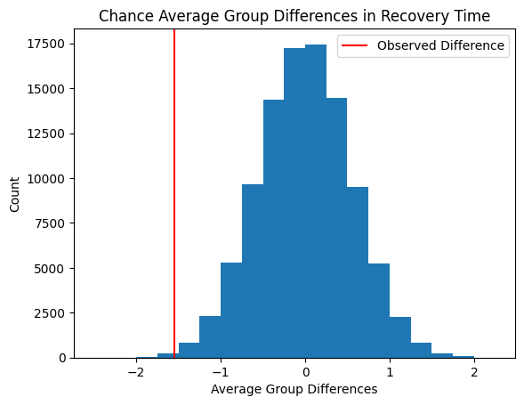
Original observed average group difference in recovery time between the drug group and the placebo group shown on the distribution of the chance average group differences. The number of chance observations with the same or lower recovery times than the originally observed will inform how likely our observation could happen by chance.
Of the \(1,000,000\) combinations randomly generated
There were \(205\) with a by chance recovery time the same or better than the originally observed 1.6 days faster
In other words, there is a 0.0205% chance that the original observation happened by dumb luck
\(\frac{205}{1000000} = 0.000205 = 0.0205\%\)
There is a roughly one in 50,000 chance this would have happened by dumb luck
This is where the idea of a probability value (p-value) comes in
There is a 0.000205 probability that the drug’s improved recovery time happened by chance
16.2.3.1. T-Tests and Mann-Whitney U tests
The permutation test is explained to provide the intuition into what p-values actually mean
In practice, using a t-test or Mann-Whitney U test is sufficient for this course
16.3. For Next Class
Although not entirely related, check out 3 Blue 1 Brown’s video on Bayes’ Rule