29. Sorting Recursively
Additional interesting sorting algorithms
Note
Most of the sorting images are taken directly from their wikipedia articles. Click the image to visit their respective pages.
29.1. Mergesort
Animation of Mergesort.
There are two important, but simple ideas at the root of mergesort
Merging two sorted lists, with the below idea, results in a single sorted list of all elements
An empty list, or a list of size 1, is sorted
29.1.1. Merging Lists
Start with two sorted lists
Create an new empty list
Compare the first elements of the two lists
Remove the smaller of the two from its list and append it to the end of the new list
Go to 3
Two Sorted Lists |
Merged List |
|---|---|
\(2, 5, 8, 9\)
\(1, 3, 4, 6, 7\)
|
|
\(2, 5, 8, 9\)
\(3, 4, 6, 7\)
|
\(1\) |
\(5, 8, 9\)
\(3, 4, 6, 7\)
|
\(1, 2\) |
\(5, 8, 9\)
\(4, 6, 7\)
|
\(1, 2, 3\) |
\(5, 8, 9\)
\(6, 7\)
|
\(1, 2, 3, 4\) |
\(8, 9\)
\(6, 7\)
|
\(1, 2, 3, 4, 5\) |
\(8, 9\)
\(7\)
|
\(1, 2, 3, 4, 5, 6\) |
\(8, 9\)
|
\(1, 2, 3, 4, 5, 6, 7\) |
\(1, 2, 3, 4, 5, 6, 7, 8, 9\) |
In the last two rows, since the second list was empty, the remainder of the first list can simply be appended to the merged list
29.1.2. Splitting Lists
The merge algorithm requires sorted lists to start merging
However, when given an unsorted collection to sort, there are no sorted lists to start merging
Fortunately this is trivial to address
Keep splitting the unsorted collection in half
Eventually this will result in a set of lists that are either empty or size 1
\([a, b, c, d, e, f, g]\)
\([a, b, c, d], [e, f, g]\)
\([a, b], [c, d], [e, f], [g]\)
\([a, b], [c, d], [e, f], [g]\)
\([a], [b], [c], [d], [e], [f], [g], []\)
29.1.3. Putting it Back Together Again
To get to the single sorted list, simply merge all the smaller sorted lists together until 1 list remains
\([t], [u], [v], [w], [x], [y], [z], []\)
\([t, u], [v, w], [x, y], [z]\)
\([t, u, v, w], [x, y, z]\)
\([t, u, v, w, x, y, z]\)
29.1.4. Recursively Thinking
The beauty of this algorithm is it’s simplicity when thinking about it recursively
 1Define Mergesort
 2    If the list is of size 0 or 1
 3        Return the sorted list of size 0 or 1
 4
 5    else
 6        Split the list into a first and second half
 7        Sort the first half with Mergesort
 8        Sort the second half with Mergesort
 9        Merge the sorted first and second halves back together
10        Return the sorted merged list
29.1.5. Complexity Analysis
A simple way to think about the analysis is to consider
How much work is involved for a single merging of two lists
How many times merging needs to happen
It can get more nuanced, but this level of detail is sufficient
29.1.5.1. Merging
Given two lists of roughly the same size \(n\) to merge into one
The algorithm compares elements and eventually adds them all to a new, sorted merged list
Interestingly, the elements in the merged list never need to be compared to one another again
The complexity of merging is \(O(n)\)
29.1.5.2. Number of Merges
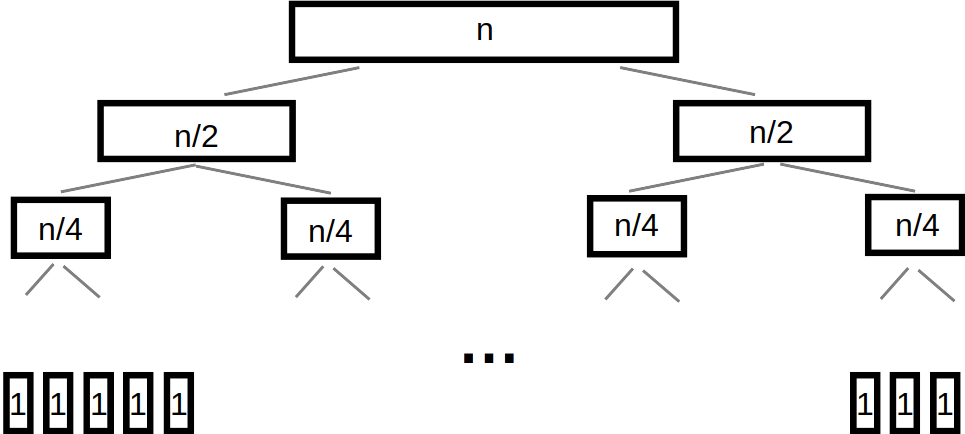
Assuming \(n\) is a power of \(2\), repeatedly splitting a list of \(n\) elements in half until \(n\) lists of size \(1\) exist.
The splitting of data can be visualized as a tree
On each level of the tree, there are a total of \(n\) elements to be merged into larger lists
Merging is \(O(n)\)
When repeatedly halving, the relationship between \(n\) and the number of levels in the tree is \(O(log_{2}(n))\)
\(O(n)\) work is required a total of \(O(log_{2}(n))\) times
Therefore mergesort is \(O(n log_{2}(n))\)
29.2. Quicksort
Animation of Quicksort.
There are two important ideas at the root of quicksort
Given a list of sorted values \(< x\), and another list of sorted values \(> x\)
The first and second lists can be concatenated to create a larger sorted list
- e.g.
\([0, 1, 2, 3, 4]\) & \([5, 6, 7, 8, 9]\)
\([0, 1, 2, 3, 4, 5, 6, 7, 8, 9]\)
An empty list, or a list of size 1, is sorted
29.2.1. Pivoting
When given an unsorted collection to sort, there are no sorted lists to start concatenating
Fortunately there is a simple way to do this
Repeat the following idea until left with lists of size 1 or 0
Select a pivot element in the list
Place all elements less than the pivot into a list
Place all elements larger than the pivot into a list
Example:
\([4, 3, 8, 6, 0, 1, 9, 2, 7, 5]\)
\([4, 3, 0, 1, 2], [5], [8, 6, 9, 7]\)
\([0, 1], [2], [4, 3], [5], [6], [7], [8, 9]\)
\([0], [1], [], [2], [], [3], [4], [5], [6], [7], [8], [9], []\)
Note that, in the above example:
For simplicity, the last element of each list was selected as the pivot
When there were no elements less than/greater than the pivot, an empty list was shown
Also notice that one could start concatenating the lists of size 1 and 0 together to result in a sorted collection
29.2.2. Recursively Thinking
 1Define Quicksort
 2    If the list is of size 0 or 1
 3        Return the sorted list of size 0 or 1
 4
 5    else
 6        Select a pivot
 7        Put all elements less than the pivot into a list
 8        Put all elements greater than the pivot into a second list
 9        Sort the first list with Quicksort
10        Sort the second list with Quicksort
11        Concatenate the sorted first list, the pivot, and the sorted second list together
12        Return the sorted concatenated list
29.2.3. Complexity Analysis
The analysis of this algorithm gets interesting since it ends up depending a lot on the pivot
29.2.3.1. Good Pivots
Assuming \(n\) is a power of \(2\), repeatedly splitting a list of \(n\) elements in half until \(n\) lists of size \(1\) exist.
If pivots are selected such that the first and second lists are roughly the same size, then the analysis ends up similar to mergesort
In other words, the pivot ends up being the median, or roughly the median value in the list
This means that roughly half the values are less than the pivot, and the other half are greater than the pivot
Like mergesort, the list sizes roughly half each time, thus the height of the tree is \(log_{2}(n)\)
\(1028 \rightarrow 512 \rightarrow 256 \rightarrow 128 \rightarrow 64 \rightarrow 32 \rightarrow 16 \rightarrow 8 \rightarrow 4 \rightarrow 2 \rightarrow 1\)
Notice in the above example, it took only 10 steps to get to 1
If it was linear, it would have taken 1027 steps
\(1028 \rightarrow 1027 \rightarrow 1026 \rightarrow 1025 \rightarrow ...\)
Concatenating these lists is linear — \(O(n)\)
Concatenation is done for each level in the tree
Therefore quicksort with good pivots is \(O(n log_{2}(n))\)
29.2.3.2. Bad Pivots
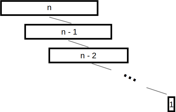
Extreme example of selecting bad pivots. If the smallest element was selected as the pivot each time, the first list would be empty and the second list would have a size of \(n - 1\). The depth of the “tree” would be \(n\).
The good pivot example assumed a pivot of roughly the median value being selected every time
Unfortunately, it is also possible that the pivot is nowhere near the median value
The above figure demonstrates what would happen if a particularly bad pivot was selected — always the smallest element in the collection
Notice that this structure looks more like a list than a tree
If it happens that there are \(0\) elements less than the pivot, and \(n-1\) elements larger, then each level of the tree only loses one element — the pivot
This means that the height of the tree is now \(n\)
Given that
Concatenating the list is linear — \(O(n)\)
Concatenation occurs for each level in the “tree”
There are a total of \(n\) levels
Therefore quicksort with bad pivots is \(O(n^{2})\)
29.2.3.3. Average Pivots
Fortunately however, always selecting bad pivots is very unlikely
In practice, quicksort is, on average, \(O(n log_{2}(n))\)
Demonstrating this can get quite complex and will not be discussed
If interested, check out the relevant wikipedia article
29.3. Heapsort
Heapsort’s magic comes from the underlying data structure — a heap
Or perhaps more accurately, a min heap
To learn about the heap data structure, see lab 10
To sort a collection of elements with a min heap, simply
Add all elements to the min heap
Remove the minimum element from the heap
Append the removed element in the sorted collection
Repeat steps 2 & 3 until the min heap is empty
29.3.1. Complexity Analysis
The whole sorting process is effectively done by the ordered property of the min heap data structure
Given \(n\) elements to be sorted, all that is needed is
Add all the elements to a min heap to build the min heap
Remove all the elements from the min heap
All \(n\) elements must be added to the min heap, and then \(n\) elements must be removed from the min heap
Thus, it becomes a matter of determining the complexity of the adding and removing to/from a min heap
29.3.1.1. Bubble Up
Every time something is added to the min heap, it may have to bubble up
The question is, how far might the element need to travel up the tree?
Fortunately this is simple to answer
If the smallest element is added to an existing min heap
It will bubble all the way to the top and be the root
Given that the heap is always a complete binary tree
And the relationship between the number of elements \(n\) in a complete binary tree and the height of the tree is \(O(log_{2}(n))\)
The complexity of bubbling up is, worst case, \(O(log_{2}(n))\)
The furthest any element may need to “bubble up” is the height of the tree
Therefore, if a total of \(n\) elements may need to bubble up to build the min heap, this has a complexity of \(O(n log_{2}(n))\)
29.3.1.2. Bubble Down
Once the min heap is created, all that’s needed is to repeatedly remove the root
But when removing, in order to maintain the min heap property, bubbling down will be required
The complexity analysis of bubbling down is more-or-less the same as bubbling up
How far may the element need to travel down the min heap?
All the way to a leaf
Given that the min heap is a complete binary tree
Bubbling down to a leaf is \(O(log_{2}(n))\)
Therefore, if removing \(n\) elements, bubble down will occur \(n\) times
\(O(n log_{2}(n))\)
29.3.1.3. Overall Complexity
Both building the min heap and removing from it are \(O(n log_{2}(n))\)
Although \(O(n log_{2}(n))\) work is happening two times, coefficients are ignored
Therefore, the computational complexity of heapsort is \(O(n log_{2}(n))\)
29.4. Radix Sort
So far, each algorithm sorts by comparing elements to other elements to determine where they should be
However, it is actually possible to sort elements without ever comparing them to any other element
The general idea is to group numbers based on individual digits
Radix means base, like base 10 numbers
Each digit is used to group the elements
It is possible to go from least significant to most significant digit, or vice versa
Here, the least significant is started with
This strategy is probably best explained with an example
Given an unsorted list, create a bin for each digit and place each element into the bin with the matching least significant digit
\(44, 33, 11, 22, 154, 10, 1, 43, 99, 47\) |
\(\{10\} \{11, 1\} \{22\} \{33, 43\} \{44, 154\} \{\} \{\} \{47\} \{\} \{99\}\) |
The next steps are to concatenate the bins and continue this process, but for each digit, moving left to right
Add leading zeros if needed
\(10, 11, 01, 22, 33, 43, 44, 154, 47, 99\) |
\(\{01\} \{10, 11\} \{22\} \{33\} \{43, 44, 47\} \{154\} \{\} \{\} \{\} \{99\}\) |
\(001, 010, 011, 022, 033, 043, 044, 047, 154, 099\) |
\(\{001, 010, 011, 022, 033, 043, 044, 047, 099\} \{154\} \{\} \{\} \{\} \{\} \{\} \{\} \{\} \{\}\) |
\(0001, 0010, 0011, 0022, 0033, 0043, 0044, 0047, 0154, 0099\) |
\(\{0001, 0010, 0011, 0022, 0033, 0043, 0044, 0047, 0099, 0154\} \{\} \{\} \{\} \{\} \{\} \{\} \{\} \{\} \{\}\) |
The algorithm finishes once all digits are used
\(1, 10, 11, 22, 33, 43, 44, 47, 99, 154\)
29.4.1. Computational Complexity
Assuming:
A collection of \(n\) things that need to be sorted
The longest number to be sorted has \(w\) symbols
E.g. the number of digits in the base 10 numbers
Each of the \(n\) elements needs to be placed in their correct bin
Assuming the use of a dictionary, this will take \(n\) \(O(1)\) operations
Therefore, \(O(n)\)
This process needs to be repeated for each symbol
\(O(n * w)\)
This is typically how the computational complexity is expressed for radix sort
It is possible that the length of the numbers \(w\) is fixed and reasonably small, so sometimes people will treat this like a constant
If one thinks of it this way, the complexity could be interpreted as \(O(n)\)
Note
The radix value does have an impact on the algorithm too (e.g. base 10 numbers vs. base 16); however, (a) it mostly impacts the space complexity, (b) it will only impact the computational complexity if a naive strategy of a linear search is used to place elements in the correct bins, and (c) the radix value is very likely to be small and fixed, thereby making it effectively a constant.
29.5. For Next Time
Read Chapter 9 Section 2
26 pages